179
CHAPTER 8
Economic Growth I: Capital
Accumulations and Population
Growth
Notes to the Instructor
Chapter Summary
These next two chapters present the Solow growth model. Although they are two of the more
difficult chapters in the book, they cover material that students usually find interesting. Chapter
8 proceeds by first holding population and technology constant and showing how the rate of
saving determines the steady–state capital–labor ratio. The chapter then discusses the positive
and normative implications of the Golden Rule level of accumulation. Following this, the model
is expanded to consider population growth. The purpose of the chapter is to teach students about
some of the determinants of economic well–being and to offer some explanations of international
differences in living standards. The three sections of the chapter teach the following lessons:
1. The rate of saving determines the size of a country’s capital stock. Increases in the saving
3. High population growth reduces steady–state income per worker because it is hard to
maintain high capital per worker when the number of workers is growing quickly.
Comments
Teaching all the material in Chapters 8 and 9 will probably require three to four lectures. An
abridged version of these chapters (presenting the basic model of the determination of the capital
stock and discussing population growth and technological progress informally) could be
presented in one to two lectures. Supplements 8–9 and 9-7 present notes to aid such a
presentation.
The lecture notes emphasize the connections between the Solow growth model and the
classical model of Chapter 3 wherever possible, reminding students that the economic forces
discussed in the classical model are still operative (for example, the real interest rate is still the
1. Interpreting a Dynamic Model
The Solow growth model is likely to be the first dynamic model that many economics students
encounter. It is worth explaining the idea of a dynamic model and making sure that students are
comfortable with time–series graphs. Students need to grasp the difference between levels and
2. Confusion Between the Population and the Labor Force
Students are sometimes troubled by the fact that the Solow model uses the terms population and
3. The Transition from F(K, L) to f (k)
Students sometimes have difficulty understanding the analysis of the Solow model in terms of
4. The Meaning of the Long Run
My students have told me that the material in the Instructor’s Resources on the subject of the
5. The Connection Between the Solow Model and the
Classical Model
Related to point 3, students may have difficulty seeing the connections between the models in
6. The Algebra of Growth Rates
Students may find the Solow model confusing if they do not understand the simple algebra of
7. Why Population Growth Reduces the Capital–Labor Ratio
by nk
The presence of the nk term in the equation governing the evolution of the capital–labor ratio can
trouble students. The simplest formal derivation of this term is probably as follows:
8. Confusion Between the Steady State and the Golden Rule
This is one of the biggest problems that students encounter. I suggest the following remedies:
(a) Downplay the discussion of the Golden Rule, perhaps presenting it less formally after
the analysis of population growth and technological progress, as in Supplement 9-7.
(b) Stress the technological nature of the Golden Rule—it can be defined independently of
any behavioral assumptions.
(c) Make sure that students understand the difference between f (k) and sf (k) in the
graphical analysis.
Use of the Web Site
The chapter exercises on the Solow growth model can seem a little intimidating to the students at
first, so it may be a good idea to focus some attention just on steady states. For example,
students could graph combinations of population growth rates and saving rates that keep output
per worker constant.
Since the Solow growth model can seem abstract to students, another idea is to calibrate
the model roughly to the U.S. economy and then ask questions about the long–run effects of
changes in saving rates such as those observed in the 1980s.
Use of the Dismal Scientist Web Site
Use the Dismal Scientist Web site to download annual data for the U.S. population 16 years and
older since 1950. Also, download annual data for real disposable personal income over the same
time period. Compute the growth rate of per–capita income on average over each decade (1950s,
1960s, etc.). Discuss changes in the growth rate of per–capita income over these decades.
Chapter Supplements
This chapter contains the following supplements:
8-1 How Long Is the Long Run? Part Two
8-2 Growth Facts
8-3 Does the Solow Model Really Explain Japanese Growth? (Case Study)
8-5 Growth Rates, Logarithms, and Elasticities
8-7 Bridge Jobs and the Transition to Retirement
8-8 How Much Variation in Per–Capita Output Is Explained by s and n? (Case Studies)
8-10 Additional Readings
182 | CHAPTER 8 Economic Growth I: Capital Accumulations and Population Growth
Lecture Notes
Introduction
Having analyzed the overall production, distribution, and allocation of national income, we now
consider the determinants of long–run growth. One stylized fact of macroeconomics is that, in
developed economies, output grows over time. This growth is irregular and is sometimes
8-1 The Accumulation of Capital
Our starting point is the production function:
Y = F(K, L).
From this equation, we see three possible sources of long–run output growth. First, the
capital stock may increase over time. Second, labor employed may change over time, perhaps as
population changes. Third, as discussed in the next chapter, the production function itself may
The Supply and Demand for Goods
Suppose that the production function has constant returns to scale. [Recall that this means that,
for any positive z, zF(K, L) = F(zK, zL).] If z = (1/L),
Y/L = F(K/L, 1).
That is, we can write the production function in per–capita terms and obtain a function of only
one variable—the capital–labor ratio—rather than two. Let y = Y/L and k = K/L, and write this as
y = f (k).
As an example, the Cobb–Douglas function Y = (KL)1/2 becomes
!
Supplement 8–1,
“How Long Is the
!Figure 8-1
!Table 8-1
Lecture Notes | 183
MPK = f (k + 1) – f (k).
As in Chapter 3, we expect the marginal product of capital to decrease as the capital–labor ratio
increases.
The Solow model is a long–run version of our previous analysis of national income and,
like that model, is based on equilibrium in the markets for goods and factors of production. For
simplicity, we suppose that there is no government (G = T = 0). We write everything in per–
capita terms: c = C/Y; i = I/Y. We have equilibrium in the market for goods:
y = c + i.
Growth in the Capital Stock in the Steady State
Investment means that the economy is acquiring new factories, machines, houses, and so forth,
which tends to increase the economy’s capital stock and allow for more production. But, at the
same time, some of these machines and factories wear out and have to be replaced. This
depreciation decreases the capital stock. If there were no investment at all, the capital stock
would decline over time. We suppose that δ percent of the capital stock wears out each period,
so if the capital stock at the start of the period is k, the depreciation during the period is δk. The
rate of depreciation can be interpreted in terms of the lifetime of the typical piece of capital. If,
say, the typical machine lasts for five years, then the depreciation rate is 20 percent (since a
factory with 100 machines would have to replace an average of 20 every year). In general, the
average lifetime of a piece of capital equals 1/ δ. For some types of capital, such as buildings, the
depreciation rate might be very low (perhaps 1 percent to 2 percent), while for, say, personal
computers, it would be much higher (perhaps 10 percent to 20 percent).
We look at a situation where the economy is in a steady state, which entails finding a
balance between the investment that is carried out in each period and the depreciation of the
capital stock that occurs over time. The overall change in the capital stock is the net effect of
new investment and depreciation:
!Figure 8-2
!Figure 8-3
184 | CHAPTER 8 Economic Growth I: Capital Accumulations and Population Growth
⇒
k* = (s/δ)2.
For example, if people save 30 percent of their income and the depreciation rate is 10 percent,
then the steady–state capital–labor ratio is (0.3/0.1)2 = 9. This illustrates two important and
intuitive results: Increases in the saving rate increase the steady–state capital–labor ratio, while
increases in the depreciation rate decrease it.
If k is at its steady–state value, it will not change. What happens if k is at some other value?
Approaching the Steady State: A Numerical Example
Consider the previous example: y = k1/2; s = 0.3; δ = 0.1. Suppose that the initial capital stock per
worker is 4. Then, output per worker equals 2, so saving per worker equals 0.6 (0.3 × 2) and
total depreciation per worker equals 0.4 (0.1 × 4). Since new investment exceeds depreciation,
Case Study: The Miracle of Japanese and German Growth
At the end of World War II, the defeated countries of Japan and Germany were in poor
economic shape because the war had destroyed a large part of their capital stocks. The Solow
growth model predicts that, if a country is in steady state and then loses a lot of its capital, it will
suffer an immediate loss in output but will also experience relatively rapid economic growth as it
builds its capital stock back up to the steady–state level. This fits the experience of Japan and
Germany in the decades immediately following World War II, when both countries exhibited
How Saving Affects Growth
The Solow growth model indicates that the saving rate is an important determinant of the steady–
state capital stock and the level of output. A country with a higher saving rate invests more and
so can sustain a higher capital stock, implying higher output in turn.
Case Study: Saving and Investment Around the World
The predicted positive relationship between saving rates and income is borne out by
international comparison. This is the first step in understanding why some countries are rich
while others are poor. The data, however, do not explain why saving and investment vary so
much across countries. Nor can the data distinguish whether high saving rates result in high
income or whether high income results in high saving rates. In addition, some countries with
very similar saving rates have very different levels of income per capita.
!Figure 8-4
!Supplement 8–3,
“Does the Solow
Method Really
Explain Japanese
Growth?”
!Figure 8-5
!Supplement 8–4,
!Figure 8-6
!Figure 8-9
8-2 The Golden Rule Level of Capital
Comparing Steady States
The steady state with the highest possible level of consumption is known as the Golden Rule
level of capital accumulation. The Golden Rule depends purely on the technological possibilities
of the economy. It can be analyzed without reference to people’s behavior (that is, without
reference to the saving rate).
At a given value of the capital–labor ratio (k), there will be depreciation equal to δk. To
maintain this level of the capital–labor ratio, an amount of output equal to δk must be set aside
for replacement investment. The output that then remains [f (k) – δk] is the level of consumption
that can be sustained at this value of k.
To identify the Golden Rule value of the capital–labor ratio, consider the effects of
changes in k on sustainable consumption. A one–unit increase in k raises output by the marginal
product of capital. It also implies that an extra δ units of output must be set aside to maintain the
Finding the Golden Rule Steady State: A Numerical Example
Policymakers who wish to influence the marginal product of capital can enact policies aimed at
influencing the saving rate.
Suppose that, by means of appropriate tax policies, the government can effectively choose
the saving rate. By an appropriate choice of s, it could place the economy at the Golden Rule.
That is, it could choose s such that the steady state of the economy (k*) corresponded to the
Golden Rule (k*
gold). For example, if y = k1/2, then the Golden Rule occurs when s = 1/2. If the
depreciation rate is 10 percent, then, at this equilibrium, k* = k*
gold = 25; y = 5; and c = 2.5.
The Transition to the Golden Rule Steady State
Suppose that policymakers decide that they would like to move the economy to the Golden Rule.
There are two possibilities: We start off either with more capital than at the Golden Rule or with
less capital than at the Golden Rule. First, consider the less realistic case, where we have more
capital than at the Golden Rule, so the saving rate is too high. Suppose that at time t0 the saving
rate is suddenly reduced. To start, we have the same amount of output and we are saving less, so
we are able to consume more immediately. Gradually, depreciation will start to eat into the
!Figure 8-7
!Figure 8-8
!Table 8-3
186 | CHAPTER 8 Economic Growth I: Capital Accumulations and Population Growth
consequence is a decline in living standards, since consumption must fall immediately, but
output will grow only slowly over time. So we trade off lower consumption in the present for
higher consumption in the future. It is not self–evident that this is desirable. Over time, people
die and new generations are born. Current generations make the sacrifice, while future
generations reap the benefit. The Golden Rule does not tell us the optimal level of capital
accumulation but simply picks out one point of interest.
8-3 Population Growth
The Solow model teaches us that we cannot explain sustained economic growth in terms of
growth in capital per worker since the economy will tend toward a steady state where capital per
worker is constant. We now consider population change as a possible explanation of sustained
economic growth.
We will assume a population growth rate equal to n. For example, if n = 0.02, then the
population increases by 2 percent every year. If it is 100 million one year, it will be 102 million
the next year. If it is 250 million this year, it will be 255 million next year.
The Steady State With Population Growth
The difference this makes to the model is that the change in the capital stock becomes
∆k = i – δk – nk,
since population growth decreases the amount of capital per worker, other things being equal. To
keep the capital–labor ratio constant, we not only need investment to replace depreciated capital,
The Effects of Population Growth
We now have an explanation for steady–state growth absent from the first version of the Solow
model. If population is growing, then in the steady state we will observe output and the capital
stock also growing at the rate n. (Recall that the production function is constant returns to scale,
which means that if K is growing at the rate n and L is growing at the rate n, then Y must also be
growing at the rate n.)
Population Growth = 0
Population Growth = n
L is constant
L grows at rate n
K is constant
K grows at rate n
k is constant
k is constant
Y is constant
Y grows at rate n
!Supplement 8–5,
“Growth Rates,
Logarithms, and
Elasticities”
Lecture Notes | 187
Case Study: Population Growth Around the World
International comparisons provide some evidence to support the prediction of the Solow model
that output and population growth are negatively related. But as in the earlier case study, the data
do not determine causality. While low population growth is associated with high income, we
cannot rule out that it is high income that reduces fertility rather than the reverse.
Alternative Perspective on Population Growth
Population growth may have additional effects beyond its interaction with capital accumulation.
Malthus, who lived in the late 1700s and early 1800s, argued that population grows at a
geometric rate while food production grows at an arithmetic rate, implying that humankind is
8-4 Conclusion
The Solow model, as developed in Chapter 8, shows how saving and population growth
!Figure 8–13
!Supplement 8–8,
“How Much
Variation in Per–
Capita Output Is
Explained by s
!Supplement 8–7,
“Bridge Jobs and
the Transition to
Retirement”
188
LECTURE SUPPLEMENT
8-1 How Long Is the Long Run? Part Two
In the Solow growth model of Chapters 8 and 9, the time horizon of the model is very different from the
classical model of Chapter 3. The classical model considers a snapshot of the economy at a point in time
(under the assumption that prices have adjusted to clear markets). The Solow growth model, by contrast,
attempts to explain the behavior of economies over many decades. Of particular note in that model is the
behavior of the capital stock through time. The capital stock is a slow–moving variable—changes in the
ADDITIONAL CASE STUDY
8-2 Growth Facts
Growth Fact Number 1
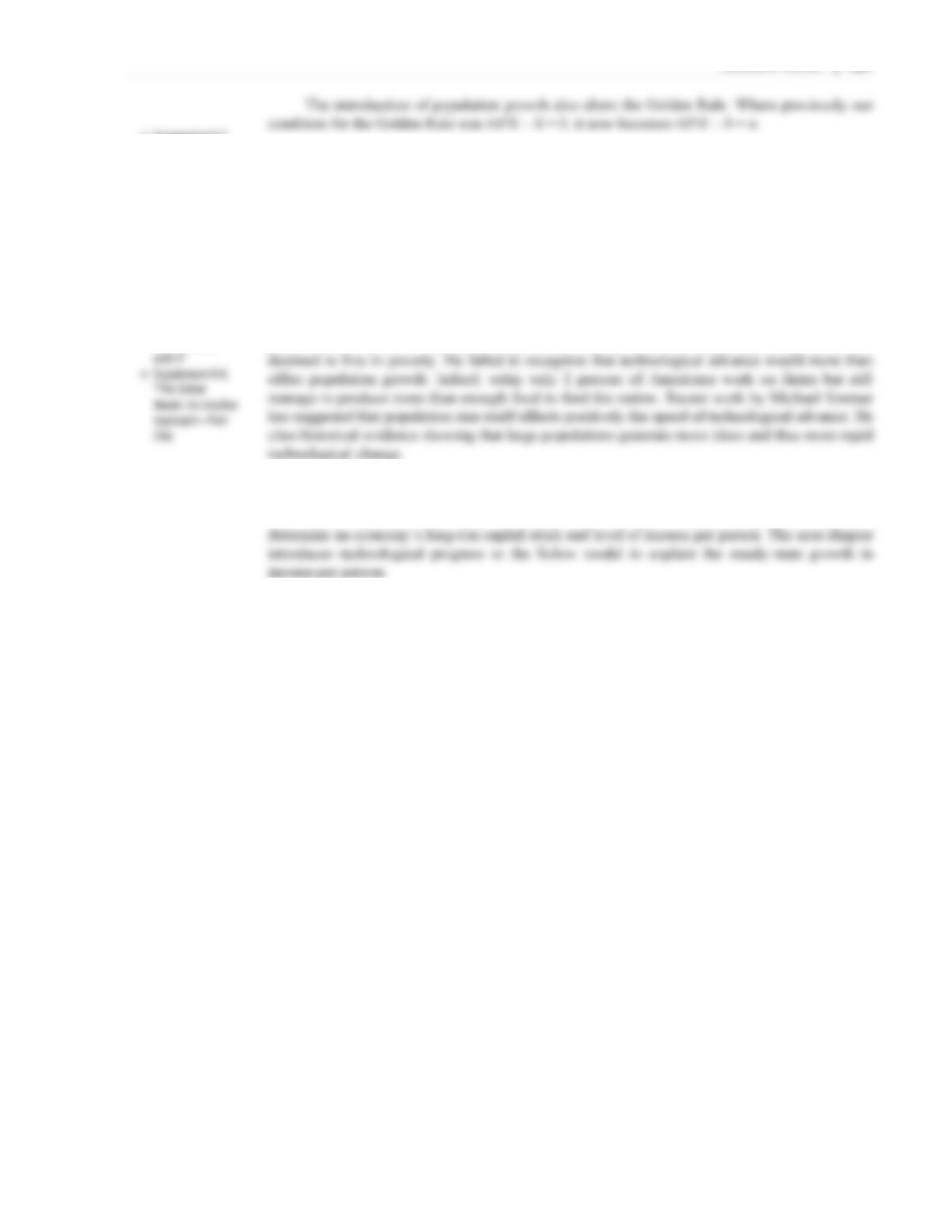
There is great income disparity among nations. This is illustrated in Figure 1, which shows that the five
poorest countries in the world possess per–capita GDP that is consistently equal to about 3 percent of U.S.
GDP per capita. This is roughly comparable to the difference in income between the most productive and
least productive workers in the United States.
Growth Fact Number 2
The evidence is mixed on whether this disparity in income is increasing or decreasing over time. If we
look at the range for the last few decades, as illustrated in Figure 1, there seems to be little change over
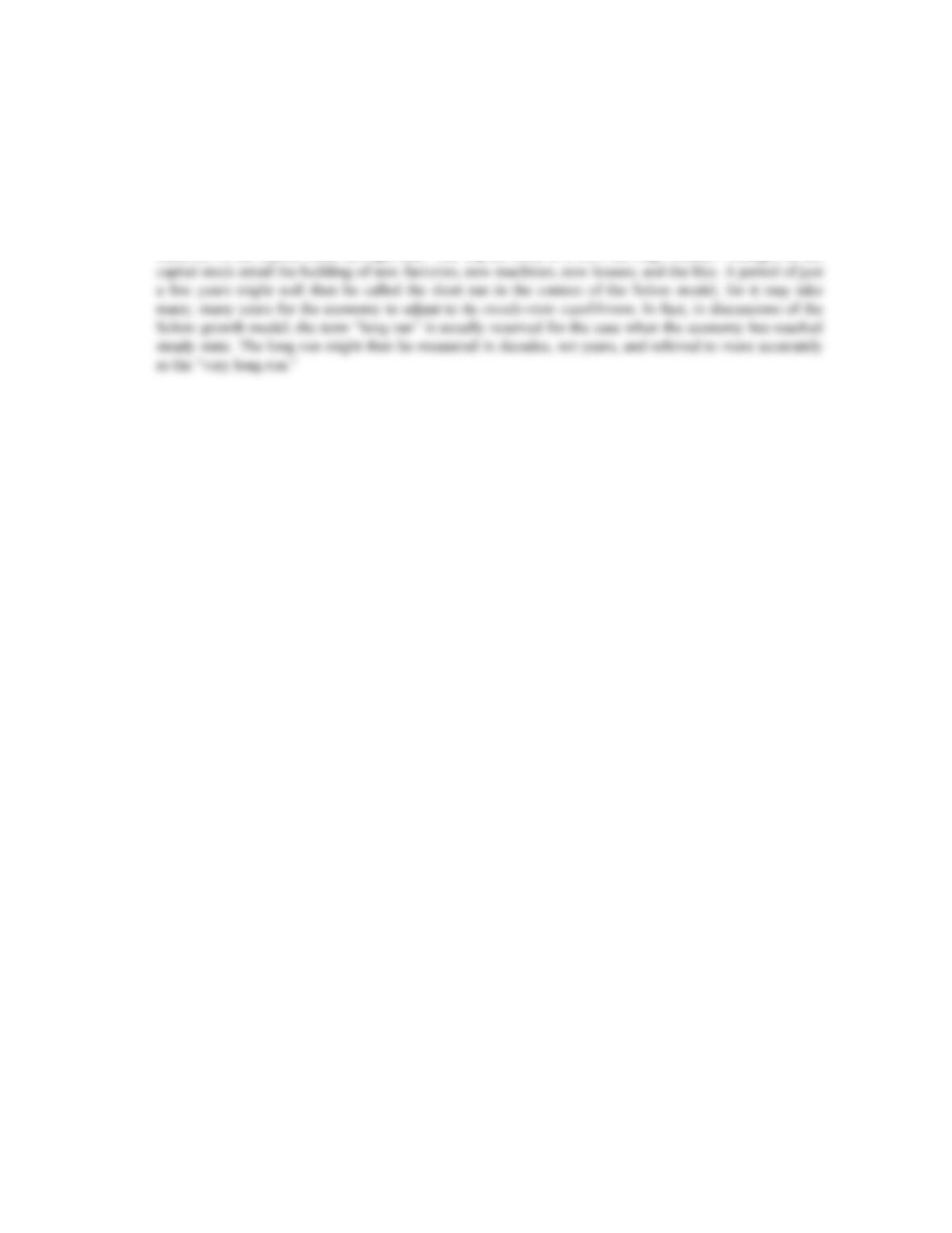
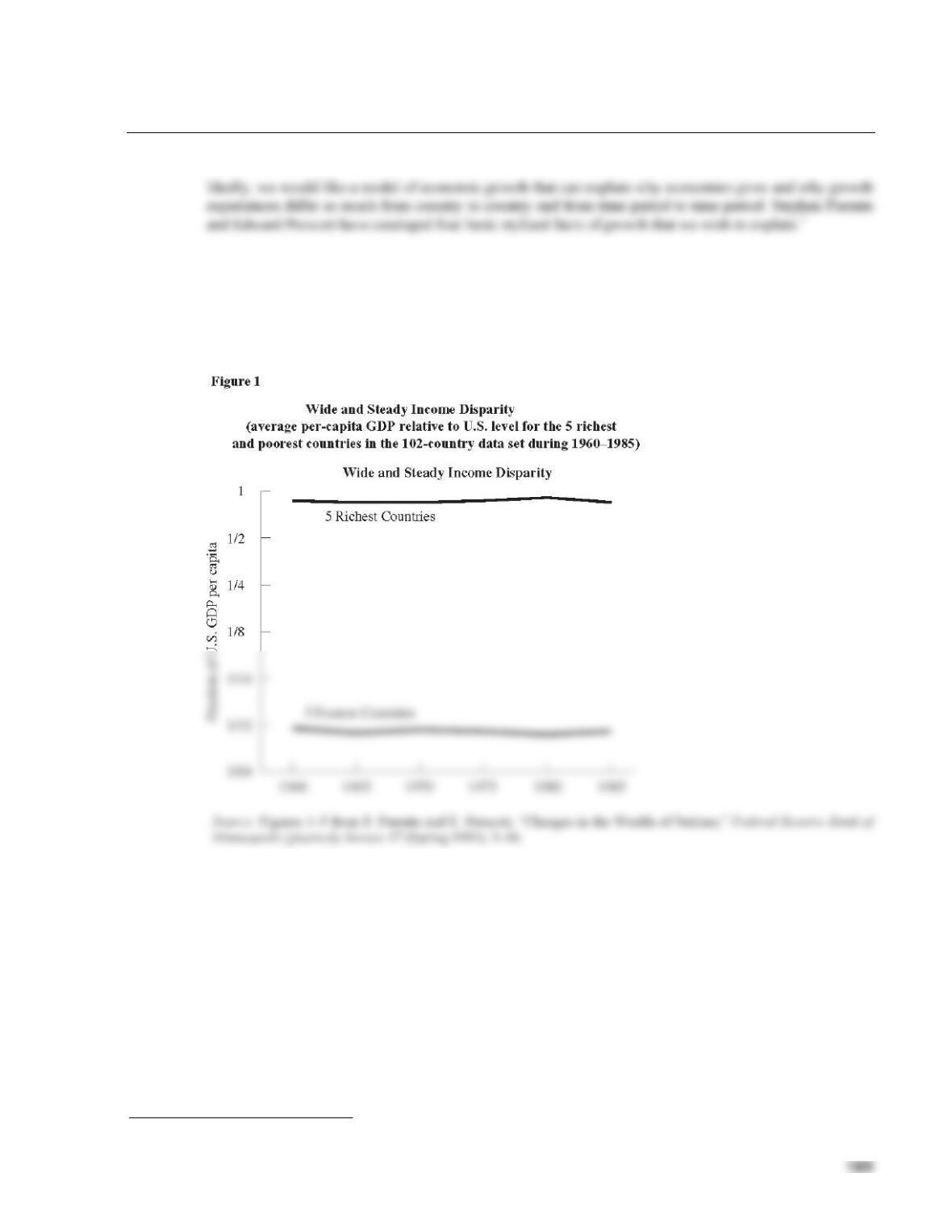
time. If we look at the standard deviation of the log of per–capita output, which provides another measure
of income dispersion, there is some slight evidence of increased disparity since 1960 (Figure 2). The
picture is different for different regions of the world: While income disparity has hardly changed in
western Europe over the last 120 years, there has been a dramatic increase in income disparity in
Southeastern Asia (Figure 3).
1 S. Parente and E. Prescott, “Changes in the Wealth of Nations,” Federal Reserve Bank of Minneapolis Quarterly Review 17 (Spring 1993): 3–16.
190
Growth Fact Number 3
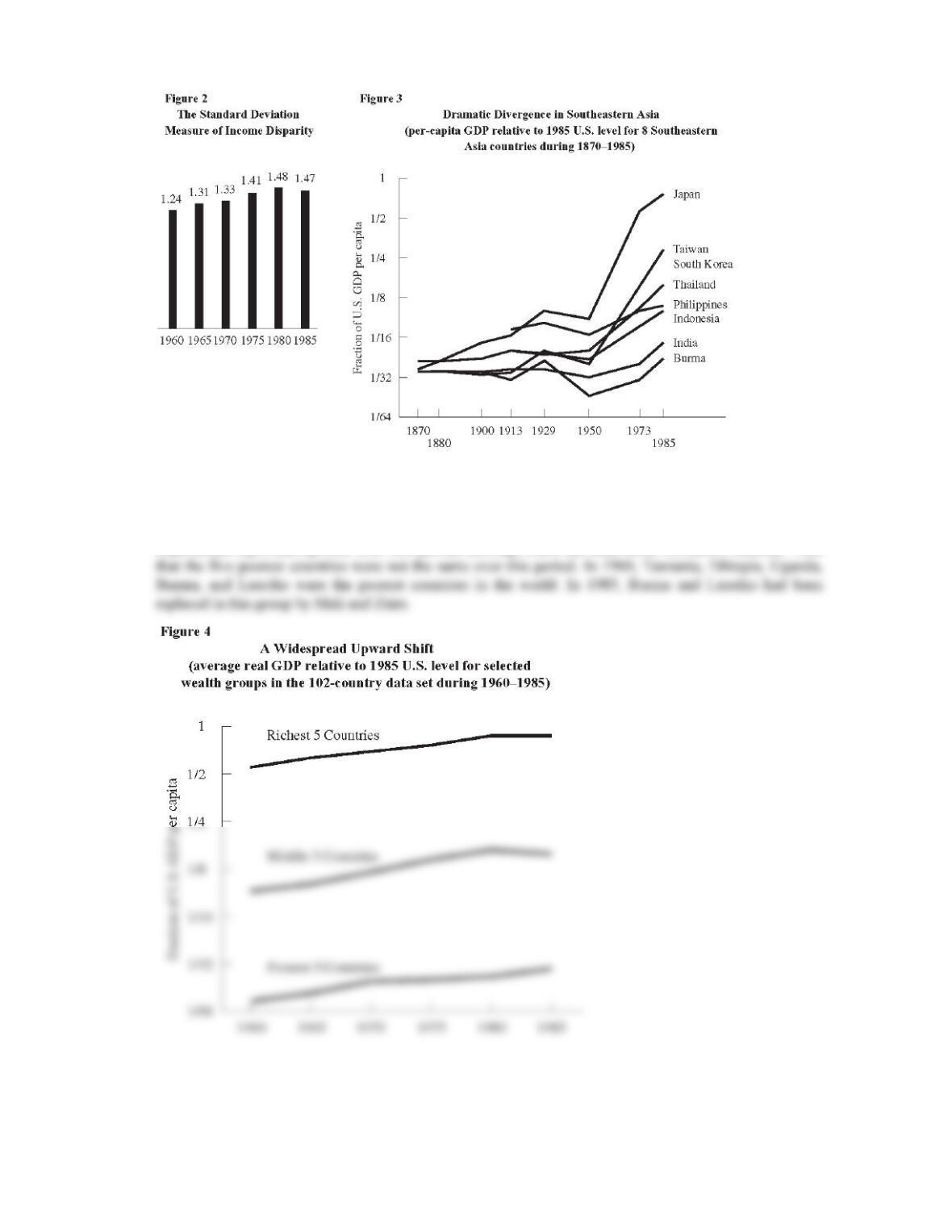
Almost all countries are getting richer. Figure 4 shows the change in per–capita GDP of the five richest
countries, the five middle countries, and the five poorest countries, between 1960 and 1985. Each group
experienced significant growth over this period, although there has been some slowdown recently. Note
191
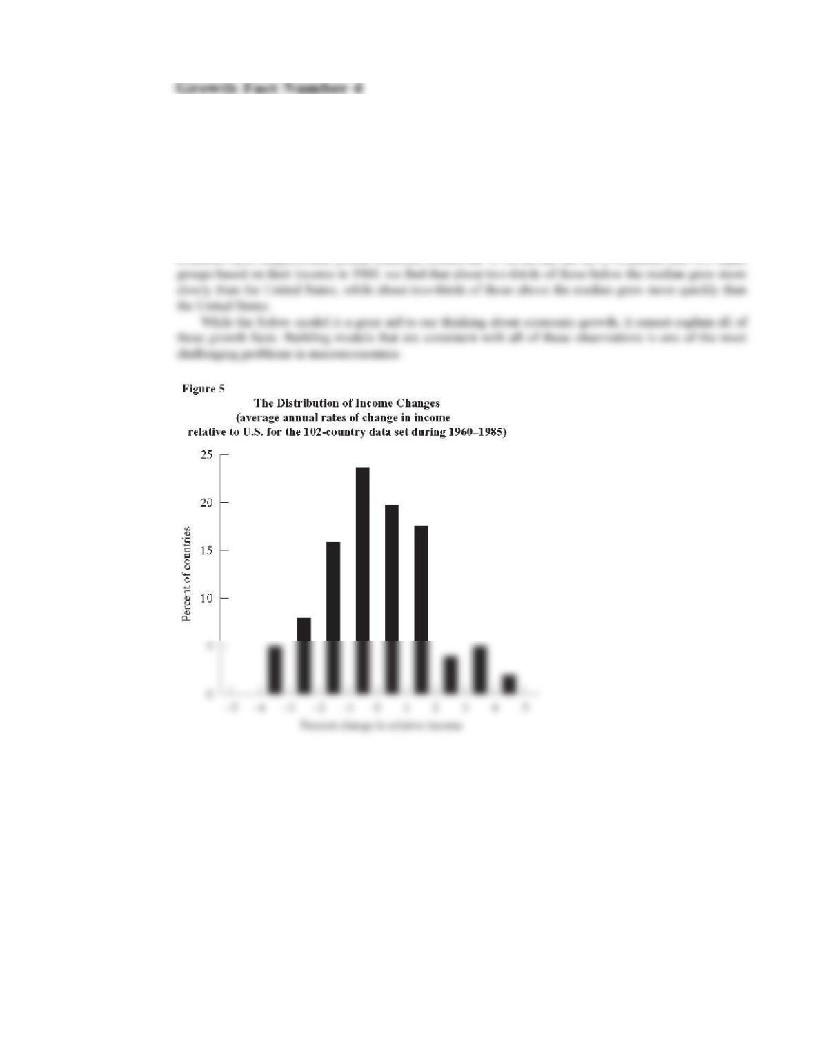
While most countries grew between 1960 and 1985, some grew at very rapid rates, while others grew
much more slowly. A few countries experienced declines. Figure 5 shows the distribution of annual
growth rates of income per capita for this period, expressed relative to the United States. The United States
grew at about 2.0 percent per annum over this period. All countries that grew at a relative rate of –2.0 or
greater thus experienced absolute increases in income. Of the 102 countries in Parente and Prescott’s data
set, all but 15 grew. Most of these were in sub–Saharan Africa. At the other end of the distribution,
countries like Taiwan and Lesotho experienced annual growth rates of real per–capita GDP of about 6
percent or more. (Recall that Lesotho was one of the five poorest countries in 1960.)
Countries, therefore, move around in the distribution of income over time. Typically, however, richer
countries have outperformed poorer countries somewhat. If we divide the set of countries into two equal
CASE STUDY EXTENSION
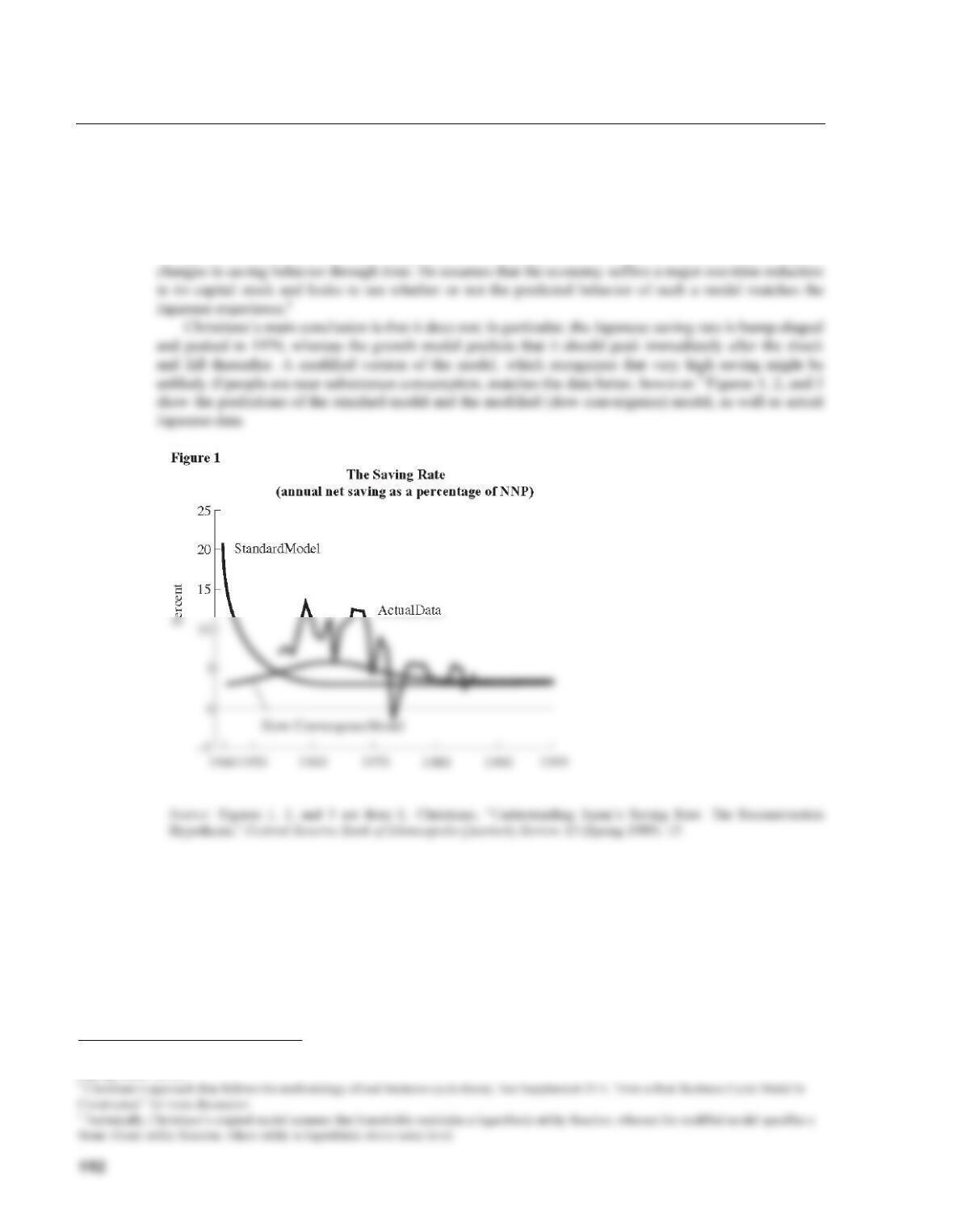
8-3 Does the Solow Model Really Explain Japanese Growth?
Lawrence Christiano has questioned whether postwar Japanese growth and saving behavior is well
explained by a simple growth model.1 He looks at the behavior of a growth model that is similar to the
Solow model, except that consumption and saving decisions are derived explicitly from optimizing
decisions of households (in contrast to the Solow model, which makes the simpler assumption that the
saving rate is constant). This extra complication is necessary because Christiano wants to try to explain
1 L. Christiano, “Understanding Japan’s Saving Rate: The Reconstruction Hypothesis,” Federal Reserve Bank of Minneapolis Quarterly Review 13
(Spring 1989): 10–25.