Questions for Review
1. In the Solow model, we find that only technological progress can affect the steady-state
rate of growth in income per worker. Growth in the capital stock (through high saving)
has no effect on the steady-state growth rate of income per worker; neither does popula-
tion growth. But technological progress can lead to sustained growth.
2. In the steady state, output per person in the Solow model grows at the rate of techno-
logical progress
g
. Capital per person also grows at rate
g
. Note that this implies that
3. To decide whether an economy has more or less capital than the Golden Rule, we need
to compare the marginal product of capital net of depreciation (MPK – δ) with the
4. Economic policy can influence the saving rate by either increasing public saving or pro-
viding incentives to stimulate private saving. Public saving is the difference between
government revenue and government spending. If spending exceeds revenue, the gov-
5. The rate of growth of output per person slowed worldwide after 1972. This slowdown
appears to reflect a slowdown in productivity growth—the rate at which the production
function is improving over time. Various explanations have been proposed, but the
slowdown remains a mystery. In the second half of the 1990s, productivity grew more
quickly again in the United States and, it appears, a few other countries. Many com-
mentators attribute the productivity revival to the effects of information technology.
6. Endogenous growth theories attempt to explain the rate of technological progress by
explaining the decisions that determine the creation of knowledge through research
and development. By contrast, the Solow model simply took this rate as exogenous. In
CHAPTER 8Economic Growth II
Problems and Applications
1. a. To solve for the steady-state value of y as a function of s, n, g, and δ, we begin with
the equation for the change in the capital stock in the steady state:
Δk= sf(k) – (δ+ n+ g)k= 0.
n= 0.01 n= 0.04
g= 0.02 g= 0.02
δ= 0.04 δ= 0.04
Using the equation for y*that we derived in part (a), we can calculate the steady-
state values of yfor each country.
2. To solve this problem, it is useful to establish what we know about the U.S. economy:
A Cobb–Douglas production function has the form y= kα, where αis capital’s share of
income. The question tells us that α= 0.3, so we know that the production function is
y= k0.3.
In the steady state, we know that the growth rate of output equals 3 percent, so we
know that (n+ g) = 0.03.
The depreciation rate δ= 0.04.
The capital–output ratio K/Y = 2.5. Because k/y = [K/(L×E)]/[Y/(L×E)] = K/Y, we
also know that k/y = 2.5. (That is, the capital–output ratio is the same in terms of
effective workers as it is in levels.)
Chapter 8 Economic Growth II 69
70 Answers to Textbook Questions and Problems
Plugging in the values established above, we find:
MPK = 0.3/2.5 = 0.12.
c. We know that at the Golden Rule steady state:
MPK = (n+ g+ δ).
Plugging in the values established above:
MPK = (0.03 + 0.04) = 0.07.
In the Golden Rule steady state, the capital–output ratio equals 4.29, compared to
the current capital–output ratio of 2.5.
e. We know from part (a) that in the steady state
s= (δ+ n+ g)(k/y),
where k/y is the steady-state capital–output ratio. In the introduction to this
the capital–output ratio is constant.
b. We know that capital’s share of income = MPK ×(K/Y). In the steady state, we
know from part (a) that the capital–output ratio K/Y is constant. We also know
from the hint that the MPK is a function of k, which is constant in the steady
state; therefore the MPK itself must be constant. Thus, capital’s share of income is
constant. Labor’s share of income is 1 – [capital’s share]. Hence, if capital’s share
is constant, we see that labor’s share of income is also constant.
Chapter 8 Economic Growth II 71
To show that the real wage wgrows at the rate of technological progress g,
define:
TLI = Total Labor Income.
L= Labor Force.
Using the hint that the real wage equals total labor income divided by the labor
force:
4. a. The per worker production function is
F(K,L)/L
=
AK
α
L
1–α
/L
=
A(K/L)
α=
Ak
α.
b. In the steady state, Δk = sf(k) – (δ+ n + g)k = 0. Hence,
sAk
α= (δ+
n
+
g
)
k
, or,
after rearranging:
c. If αequals 1/3, then Richland should be 41/2, or two times, richer than Poorland.
d. If = 16, then it must be the case that , which in turn requires that
αequals 2/3. Hence, If the Cobb-Douglas production function puts 2/3 of the
weight on capital and only 1/3 on labor, then we can explain a 16-fold difference in
levels of income per worker. One way to justify this might be to think about capital
more broadly to include human capital—which must also be accumulated through
investment, much in the way one accumulates physical capital.
k sA
n+ g
* = +
⎡
⎣
⎢⎤
⎦
⎥
1−
⎛
⎝
⎜⎞
⎠
⎟
δ
1
α
41
α
α−
⎛
⎝
⎜⎞
⎠
⎟
α
α1−
⎛
⎝
⎜⎞
⎠
⎟=2
72 Answers to Textbook Questions and Problems
5. How do differences in education across countries affect the Solow model? Education is
one factor affecting the efficiency of labor, which we denoted by E. (Other factors affect-
ing the efficiency of labor include levels of health, skill, and knowledge.) Since country
1 has a more highly educated labor force than country 2, each worker in country 1 is
more efficient. That is, E1> E2. We will assume that both countries are in steady state.
rate of population growth and the same rate of technological progress.
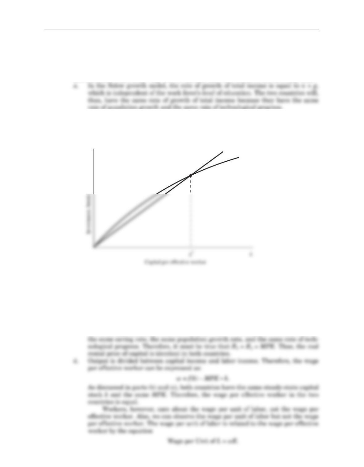
b. Because both countries have the same saving rate, the same population growth
rate, and the same rate of technological progress, we know that the two countries
will converge to the same steady-state level of capital per effective worker k*. This
is shown in Figure 8–1.
Hence, output per effective worker in the steady state, which is y*= f(k*), is the
same in both countries. But y*= Y/(L×E) or Y/L = y*E. We know that y*will be
the same in both countries, but that E1> E2. Therefore, y*E1> y*E2. This implies
that (Y/L)1> (Y/L)2. Thus, the level of income per worker will be higher in the
country with the more educated labor force.
c. We know that the real rental price of capital Requals the marginal product of cap-
ital (MPK). But the MPK depends on the capital stock per efficiency unit of labor.
In the steady state, both countries have k*
1= k*
2= k*because both countries have
(
δ
+ n + g) k
sf (k)
Figure 8–1
Thus, the wage per unit of labor is higher in the country with the more educated
labor force.
6. a. In the two-sector endogenous growth model in the text, the production function for
manufactured goods is
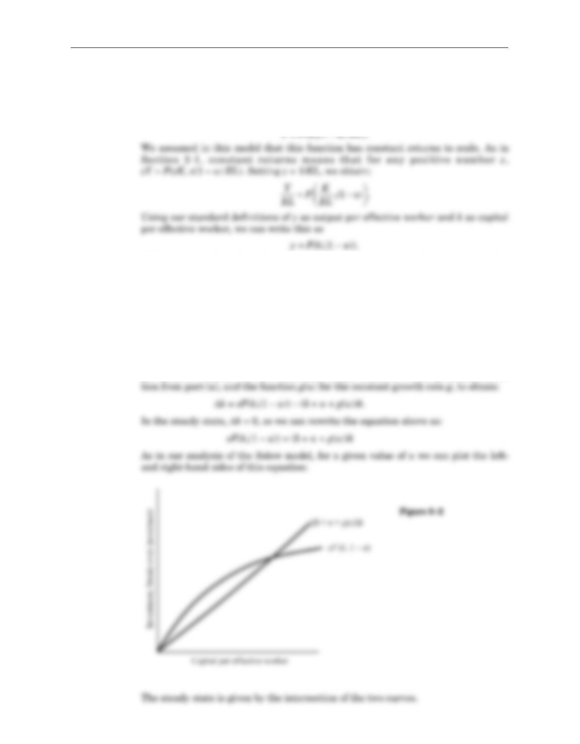
b. To begin, note that from the production function in research universities, the
growth rate of labor efficiency, ΔE/ E, equals g(u). We can now follow the logic of
Section 8-1, substituting the function g(u) for the constant growth rate g. In order
to keep capital per effective worker (K/EL) constant, break-even investment
includes three terms: δkis needed to replace depreciating capital, nk is needed to
provide capital for new workers, and g(u) is needed to provide capital for the
greater stock of knowledge Ecreated by research universities. That is, break-even
investment is (δ+ n + g(u))k.
c. Again following the logic of Section 8-1, the growth of capital per effective worker
is the difference between saving per effective worker and break-even investment
per effective worker. We now substitute the per-effective-worker production func-
Chapter 8 Economic Growth II 73
d. The steady state has constant capital per effective worker kas given by Figure
8–2 above. We also assume that in the steady state, there is a constant share of
time spent in research universities, so uis constant. (After all, if uwere not con-
rises.
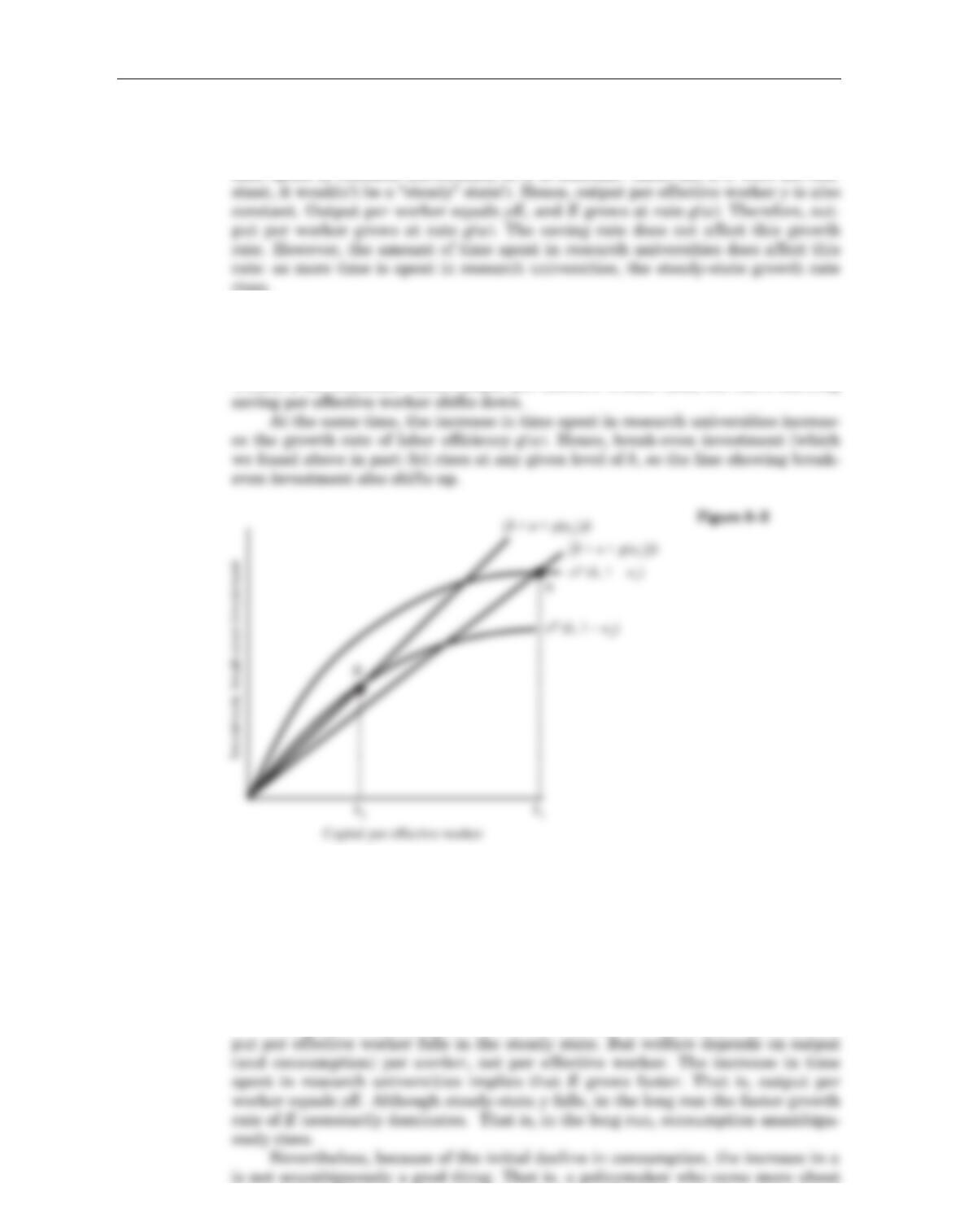
e. An increase in ushifts both lines in our figure. Output per effective worker falls
for any given level of capital per effective worker, since less of each worker’s time
is spent producing manufactured goods. This is the immediate effect of the
change, since at the time urises, the capital stock Kand the efficiency of each
worker Eare constant. Since output per effective worker falls, the curve showing
Figure 8–3 below shows these shifts:
In the new steady state, capital per effective worker falls from k1to k2. Output per
effective worker also falls.
f. In the short run, the increase in uunambiguously decreases consumption. After
all, we argued in part (e) that the immediate effect is to decrease output, since
workers spend less time producing manufacturing goods and more time in
research universities expanding the stock of knowledge. For a given saving rate,
the decrease in output implies a decrease in consumption.
The long-run steady-state effect is more subtle. We found in part (e) that out-
74 Answers to Textbook Questions and Problems
More Problems and Applications to Chapter 8
1. a. The growth in total output (Y) depends on the growth rates of labor (L), capital
(K), and total factor productivity (A), as summarized by the equation:
= 1.67%.
A 5-percent increase in labor input increases output by 1.67 percent.
Labor productivity is Y/L. We can write the growth rate in labor productivi-
ty as
= 0.
Total factor productivity is the amount of output growth that remains after we
have accounted for the determinants of growth that we can measure. In this case,
there is no change in technology, so all of the output growth is attributable to mea-
sured input growth. That is, total factor productivity growth is zero, as expected.
b. Between years 1 and 2, the capital stock grows by 1/6, labor input grows by 1/3,
and output grows by 1/6. We know that the growth in total factor productivity is
given by
Chapter 8 Economic Growth II 75
Using the mathematical trick in the hint, we can rewrite this as
= + .
Using the same trick we used above, we can express the term in brackets as
ΔK/K – ΔL/L = Δ(K/L)/(K/L).
Making this substitution in the equation for labor productivity growth, we conclude
that
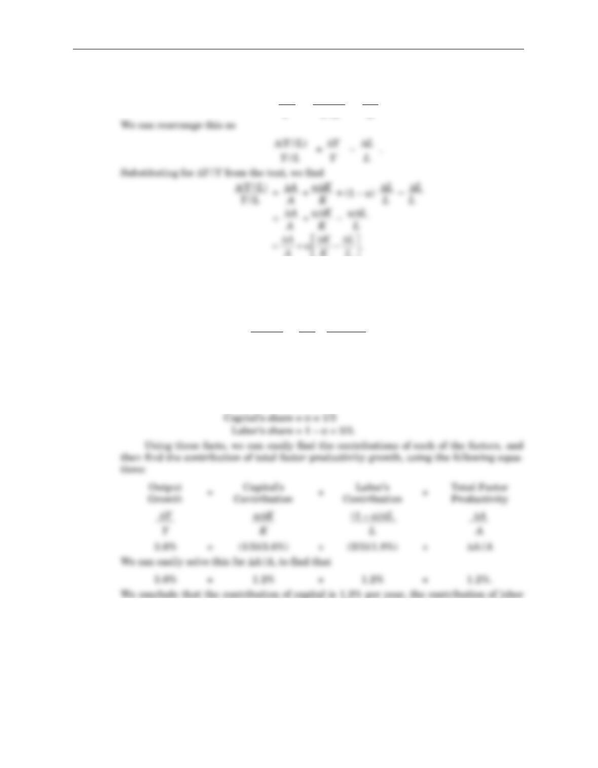
3. We know the following:
ΔY/Y = n+ g= 3.6%
ΔK/K = n+ g= 3.6%
ΔL/L = n= 1.8%
is 1.2% per year, and the contribution of total factor productivity growth is 1.2% per
year. These numbers match the ones in Table 8–3 in the text for the United States from
1948–2002.
76 Answers to Textbook Questions and Problems
Δ(Y/L) =ΔA+αΔ(K/L) .
Y/L A K/L
⎣
⎦
A
K
L
ΔY
Y
ΔL
L
Δ(Y/L)
Y/L