Chapter 8
Business Cycles
◼ Learning Objectives
I. Goals of Part 3
A. What causes business cycles?
B. How should policymakers respond to cyclical fluctuations?
C. Coverage of Chapters 8 to 11
1. Business cycle facts and features (Ch. 8)
II. Goals of Chapter 8
A. Define and describe the business cycle (Sec. 8.1)
III. Notes to Eighth Edition Users
A. This is a chapter with a lot of data, so the main change is to update all the data
Chapter 8 Business Cycles 161
◼ Teaching Notes
I. What Is a Business Cycle? (Sec. 8.1)
A. U.S. research on cycles began in 1920 at the National Bureau of Economic Research (NBER)
1. NBER maintains the business cycle chronology—a detailed history of business cycles
Data Application
A major compendium of studies on the business cycle was produced by the NBER in 1986, The
American Business Cycle: Continuity and Change, edited by Robert J. Gordon, Chicago:
University of Chicago Press. It contains general discussions of the then-current state of
B. Burns and Mitchell (Measuring Business Cycles, 1946) make five main points about
business cycles:
1. Business cycles are fluctuations of aggregate economic activity, not a specific variable
2. There are expansions and contractions
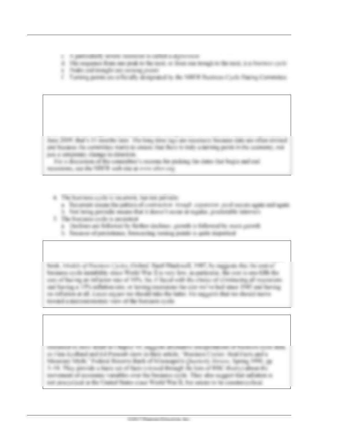
a. Aggregate economic activity declines in a contraction or recession until it reaches a
trough (Figure 8.1)
162 Abel/Bernanke/Croushore • Macroeconomics, Ninth Edition
b. Then activity increases in an expansion or boom until it reaches a peak
Data Application
The NBER Business Cycle Dating Committee must wait for some time to pass before they can
declare the start or end of a recession. For example, in the latest recession, the committee
announced in November 2008 that the recession had begun in December 2007; that’s 11 months
after the recession began. And they announced in September 2012 that the recession had ended in
3. Economic variables show comovement—they have regular and predictable patterns of
behavior over the course of the business cycle
Theoretical Application
Should we even care about the business cycle? Robert Lucas doesn’t think so. In his provocative
Data Application
New economic theories and statistical techniques may change somewhat the way in which we
look at data on the business cycle. The real business cycle (RBC) approach, which will be
Chapter 8 Business Cycles 163
II. The American Business Cycle: The Historical Record (Sec. 8.2)
A. Text Table 8.1 gives the NBER business cycle chronology
B. The pre–World War I period
1. Recessions were common from 1865 to 1917, with 338 months of contraction and
C. The Great Depression and World War II
1. The worst economic contraction was the Great Depression of the 1930s
a. Real GDP fell nearly 30% from the peak in August 1929 to the trough in March 1933
f. In 1939 the unemployment rate was over 17%
2. The Great Depression ended with the start of World War II
a. Wartime production brought the unemployment rate below 2%
b. Real GDP almost doubled between 1939 and 1944
D. Post–World War II business cycles
1. From 1945 to 1970 there were five mild contractions
2. A very long expansion (106 months, from February 1961 to December 1969) made some
E. The long boom
1. From 1982 to 2001, there was only one brief recession, from July 1990 to March 1991,
Data Application
When the expansion of the 1990s became the longest in U.S. history in early 2000, the Wall
F. The Great Recession
1. The longest and deepest recession since the Great Depression began in December 2007
a. The Great Recession began with a housing crisis (described in Chapter 7)
164 Abel/Bernanke/Croushore • Macroeconomics, Ninth Edition
Data Application
For an examination of how various macroeconomic variables, especially consumer spending,
G. Have American business cycles become less severe?
1. Economists believed that business cycles weren’t as bad after World War II as they were
before
5. New research has focused on the reasons for the decline in the volatility of U.S. output
a. Stock and Watson’s research showed that the decline came from a sharp drop in volatility
around 1984 for many economic variables; dubbed the Great Moderation
b. A plot of real GDP growth (text Figure 8.2) shows that the quarterly growth rate of GDP
6. After showing that many theories for the reduced volatility in output were not convincing,
Stock and Watson found three factors that were important
a. Reductions in the volatility of food and other commodity prices account for about 15% of
7. It is not yet clear if the Great Recession implies that the Great Moderation has ended,
though the decline in volatility in 2014 suggests that perhaps the Great Moderation is
continuing
166 Abel/Bernanke/Croushore • Macroeconomics, Ninth Edition
Data Application
Frank Diebold and Glenn Rudebusch argue that although the debate between Romer and others
III. Business Cycle Facts (Sec. 8.3)
A. All business cycles have features in common
B. The cyclical behavior of economic variables—direction and timing
1. What direction does a variable move relative to aggregate economic activity?
2. What is the timing of a variable’s movements relative to aggregate economic activity?
a. Leading: in advance
Data Application
Your students may enjoy looking at macro data on their own to see what’s out there. Some good
C. Cyclical behavior of key macroeconomic variables (text Figures 8.4 to 8.12)
1. Procyclical
Analytical Problem 3 looks at whether output or total hours worked is more volatile, given that
average labor productivity is procyclical.
2. Countercyclical: unemployment (timing is unclassified)
3. Acyclical: real interest rates (timing is not designated)
Chapter 8 Business Cycles 167
Analytical Problem 2 asks for an explanation of why expenditures on durable goods are more
volatile over the business cycle than expenditures on nondurables and services.
D. International aspects of the business cycle
1. The cyclical behavior of key economic variables in other countries is similar to that in the
United States
Data Application
For a basic set of facts about business cycles across countries, see the article by Mario J.
Crucini, M. Ayhan Kose, and Christopher Otrok, “What Are the Driving Forces of International
Business Cycles?” Review of Economic Dynamics, 2011, pp. 156–175.
E. In touch with data and research—coincident and leading indexes
1. Coincident indexes are designed to help figure out the current state of the economy, while
6. The Conference Board produces an index of leading economic indicators; a decline in the
index for two or three months in a row warns of recession danger
7. Problems with the leading indicators
a. Data are available promptly, but often revised later, so the index may give
misleading signals
b. The index has given a number of false warnings
168 Abel/Bernanke/Croushore • Macroeconomics, Ninth Edition
10. After the fact, the index of leading indicators is revised and appears to have predicted the
recessions well
11. Stock and Watson attempted to improve the index by creating some new indexes based on
12. Because recessions may be caused by sudden shocks, the search for a good index of leading
indicators may be fruitless
F. In touch with data and research: the seasonal cycle and the business cycle
Data Application
A further discovery made by Barsky and Miron in looking at the seasonal cycle is surprising:
they found little production smoothing. Economic theory suggests that even if demand changes
4. If the seasonal cycle is like the business cycle, and the seasonal cycle represents desirable
responses to various factors (Christmas, the weather) for which government intervention is
inappropriate, should government intervention be used to smooth out the business cycle?
Policy Application
Some economists have gone so far as far as to challenge the need for the Fed to change the
money supply over the seasons. If the Fed did not increase the money supply in the fall, for
example, the seasonal demand for currency due to holiday shopping would cause interest rates to
IV. Business Cycle Analysis: A Preview (Sec. 8.4)
A. What explains business cycle fluctuations?
1. Two major components of business cycle theories
2. Two major business cycle theories
3. Study both theories in aggregate demand-aggregate supply (AD–AS) framework

Chapter 8 Business Cycles 169
B. Aggregate demand and aggregate supply: a brief introduction
1. The model (along with the building block IS–LM model) will be developed in Chapters 9–11
c. Long-run aggregate supply curve
3. Aggregate demand curve
a. Shows quantity of goods and services demanded (Y) for any price level (P)
4. Aggregate supply curve
a. The aggregate supply curve shows how much output producers are willing to supply at
any given price level
Figure 8.2
(1) Short-run equilibrium: the aggregate demand curve intersects the short-run aggregate
supply curve
(2) Long-run equilibrium: the aggregate demand curve intersects the long-run aggregate
supply curve
C. Aggregate demand shocks

170 Abel/Bernanke/Croushore • Macroeconomics, Ninth Edition
Figure 8.3
a. The aggregate demand curve shifts down and to the left
b. Short-run equilibrium occurs where the aggregate demand curve intersects the short-run
3. How long does it take to get to the long run?
a. Classical theory: prices adjust rapidly
(1) So recessions are short-lived
D. Aggregate supply shocks
1. Classicals view aggregate supply shocks as the main cause of fluctuations in output
2. Example: a negative aggregate supply shock (Figure 8.4, like text Figure 8.18)

Chapter 8 Business Cycles 171
3. Keynesians also recognize the importance of supply shocks; their views are discussed further
in Chapter 11
Policy Application
In his article, “Productivity Growth and the American Business Cycle,” Federal Reserve Bank of
172 Abel/Bernanke/Croushore • Macroeconomics, Ninth Edition
◼ Additional Issues for Classroom Discussion
1. Should the Government Try to Prevent Recessions?
Ask your class if they think the government should try to prevent recessions. Most people do, but some
done nothing at all.
2. Should Government Policy Prevent the Seasonal Cycle?
Most of the data that economists look at has been adjusted to remove seasonal influences. For example, the
3. Do Recessions Have Any Positive Economic Effects?
Recessions cause hardships to many people who lose their jobs or whose incomes decline. The entire
economy slows down, making it harder for people to change jobs or for college and high-school graduates
to find jobs. Many small businesses fail, and people who had planned to open businesses wait until times
are better.
Are there any benefits to recessions? Can you think of any ways in which recessions help consumers?
What about corporations? Small business firms? Workers?
Your students may have trouble coming up with anything positive about recessions. But some new
Chapter 8 Business Cycles 173
◼ Answers to Textbook Problems
Review Questions
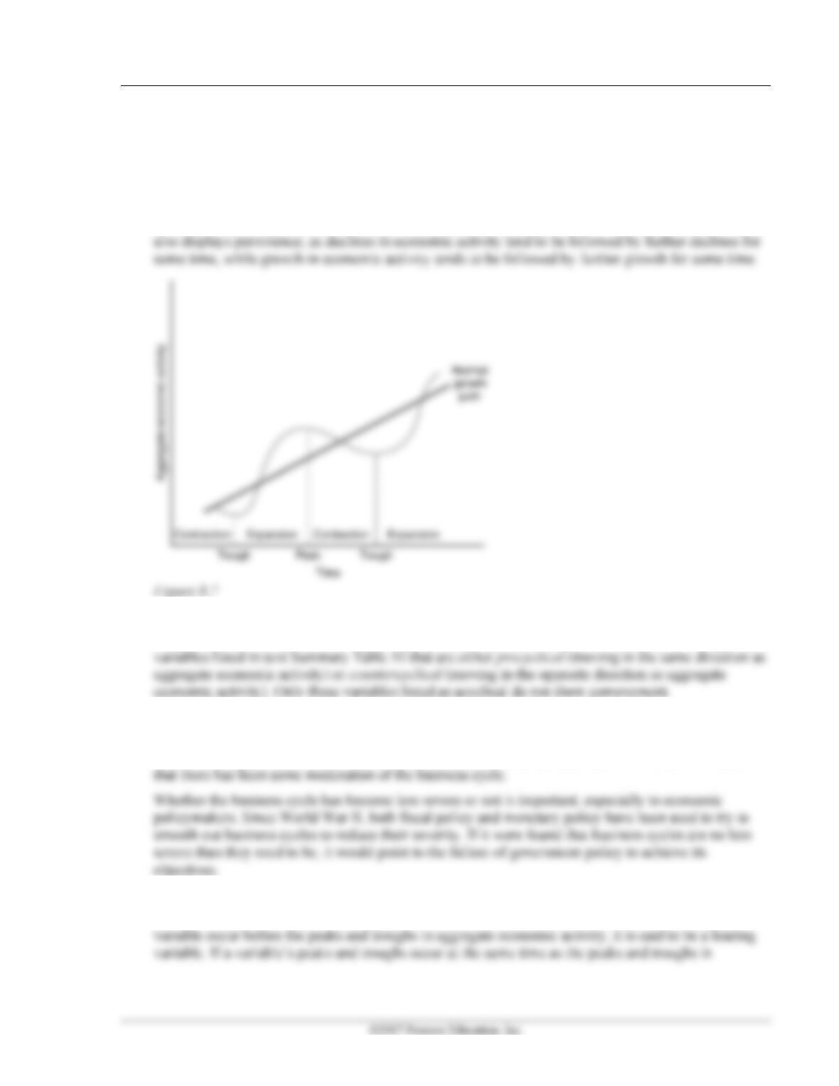
1. Figure 8.7 illustrates both the recurrence and persistence of the business cycle. The business cycle is
recurrent, as there are repeated episodes of contractions and expansions over time. The business cycle
2. Comovement means that many economic variables move together in a predictable way over the
business cycle. The business cycle facts presented in the chapter illustrate comovement among all the
3. There is some question as to whether or not the business cycle has become less volatile over time.
Originally it was thought that the cycle had been moderated, especially since World War II, but
Romer challenged this notion. Further examination of the data by Balke and Gordon, however, shows
4. A variable that moves in the same direction as aggregate economic activity is said to be procyclical,
while a variable that moves in the opposite direction is countercyclical. If the peaks and troughs of a
174 Abel/Bernanke/Croushore • Macroeconomics, Ninth Edition
5. If the economy were entering a recession, you’d expect production, investment, average labor
7. The two components of a theory of business cycles are: (1) A description of the types of factors
8. Keynesians and classicals differ sharply in their beliefs about how long it takes the economy to reach
a long-run equilibrium. Classical economists believe that prices adjust rapidly (within a few months)
to restore equilibrium in the face of a shock, while Keynesians believe that prices adjust slowly,
taking perhaps several years.
Chapter 8 Business Cycles 175
Analytical Problems
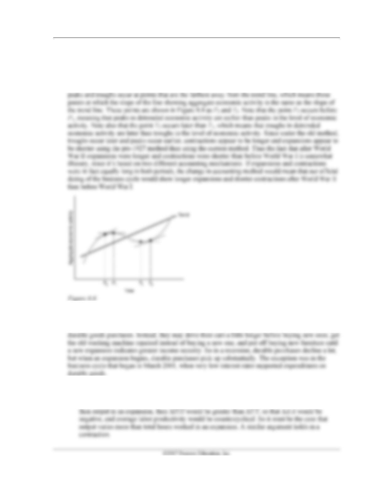
1. Figure 8.8 illustrates the business cycle. The current NBER method picks peaks and troughs in the
level of aggregate economic activity, which are points on the figure where the slope of the line is
zero. These are shown in Figure 8.8 as P1 (at the peak of the cycle) and T1 (at the trough of the cycle).
However, the older method picks peaks and troughs in detrended economic activity. This means the
2. Expenditure on durable goods is more sensitive to the business cycle than expenditure on nondurable
goods and services, because people can more easily change the timing of their expenditure on durables.
When economic activity is weak, and people face the danger of losing their jobs, they avoid making
3. (a) In symbols, let A = average labor productivity, Y = output, and H = total hours worked. By
definition, A = Y/H, so in growth terms, A/A = Y/Y − H/H. Since all three are procyclical,
they all move in the same direction over the business cycle. If total hours worked varied more
176 Abel/Bernanke/Croushore • Macroeconomics, Ninth Edition
(b) That average labor productivity is procyclical helps explain why the Okun’s Law coefficient is 2,
not 1. A one-percentage point increase in unemployment is approximately a one percent fall in
employment. Thus, if there were no change in average labor productivity, we might expect the
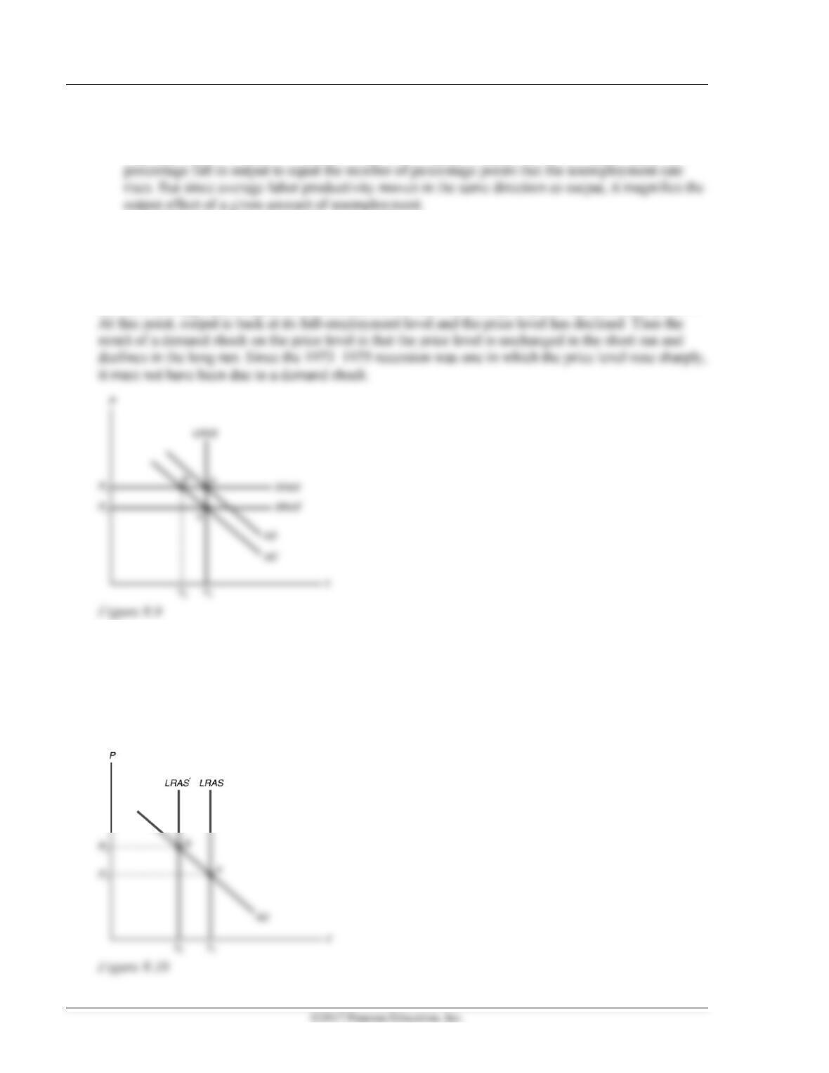
4. Figure 8.9 illustrates the effects of a demand shock. The economy begins in equilibrium at point A,
where the LRAS, SRAS, and AD curves intersect. The demand shock shifts the aggregate demand
curve to the left to AD. In the short run, the equilibrium is at point B, where AD intersects SRAS.
This is a point at which output has declined (a recession), but the price level is unchanged. Over time,
the short-run aggregate supply curve shifts down to SRAS, restoring long-run equilibrium at point C.
Figure 8.10 illustrates the effects of a supply shock. The economy begins in equilibrium at point A,
where the LRAS, SRAS, and AD curves intersect. The supply shock shifts the long-run aggregate
supply curve to the left to LRAS. The new equilibrium is at point B, where AD intersects LRAS. This
is a point at which output has declined (a recession), but the price level has risen. This matches what
happened in the 1973–1975 recession. Thus we conclude that the 1973–1975 recession was the result
of a supply shock, not a demand shock.

Chapter 8 Business Cycles 177
5. Growth that is “too rapid” most likely refers to a situation in which the aggregate demand curve has
shifted to the right and, in the short run, intersects the SRAS curve at a level of output that’s greater
than the full-employment level of output (Figure 8.11). This situation is associated with inflation
because, in the long run, prices will rise, shifting the SRAS curve up to intersect with the LRAS and
AD curves. The shock that is implicitly assumed to be hitting the economy is an aggregate demand
shock, since that’s the only shock that increases output in the short run and inflation in the long run.
Working with Macroeconomic Data
1. The unemployment rate is a persistent variable because most changes by 0.2 percentage points or more
were followed in the subsequent quarter by another change in the same direction.
2. a. Real imports are procylical and coincident.
b. Federal government receipts are procylical and coincident.
4. The business cycles of the United States and Canada are most closely related. Business cycles are
5. Many answers are possible depending on the variable chosen.