CHAPTER 7
TEACHING NOTES
This is a fairly standard chapter on using qualitative information in regression analysis, although
I try to emphasize examples with policy relevance (and only cross-sectional applications are
included.).
athlete GPAs in the text.) From a practical perspective, it is important to know whether the
partial effects differ across groups or whether a constant differential is sufficient.
I admit that an unconventional feature of this chapter is its introduction of the linear probability
model. I cover the LPM here for several reasons. First, the LPM is being used more and more
because it is easier to interpret than probit or logit models. Plus, once the proper parameter
A useful modification of the LPM estimated in equation (7.29) is to drop kidsge6 (because it is
not significant) and then define two dummy variables, one for kidslt6 equal to one and the other
for kidslt6 at least two. These can be included in place of kidslt6 (with no young children being
the base group). This allows a diminishing marginal effect in an LPM. I was a bit surprised
when a diminishing effect did not materialize.
72
SOLUTIONS TO PROBLEMS
7.1 (i) The coefficient on male is 87.75, so a man is estimated to sleep almost one and one-half
hours more per week than a comparable woman. Further, tmale = 87.75/34.33 2.56, which is
close to the 1% critical value against a two-sided alternative (about 2.58). Thus, the evidence for
7.2 (i) If cigs = 10 then
log( )bwght
= −.0044(10) = −.044, which means about a 4.4% lower
birth weight.
(ii) A white child is estimated to weigh about 5.5% more, other factors in the first equation
7.3 (i) The t statistic on hsize2 is over four in absolute value, so there is very strong evidence that
it belongs in the equation. We obtain this by finding the turnaround point; this is the value of
73
(iv) We plug in black = 1, female = 1 for black females and black = 0 and female = 1 for
nonblack females. The difference is therefore –169.81 + 62.31 = −107.50. Because the estimate
7.4 (i) The approximate difference is just the coefficient on utility times 100, or –28.3%. The t
statistic is −.283/.099 −2.86, which is very statistically significant.
7.5 (i) Following the hint,
colGPA
=
0
ˆ
+
0
ˆ
(1 – noPC) +
1
ˆ
hsGPA +
2
ˆ
ACT = (
0
ˆ
+
0
ˆ
) −
7.6 In Section 3.3 – in particular, in the discussion surrounding Table 3.2 – we discussed how to
determine the direction of bias in the OLS estimators when an important variable (ability, in this
74
7.7 (i) Write the population model underlying (7.29) as
inlf =
0
+
1
nwifeinc +
2
educ +
3
exper +
4
exper2 +
5
age
+
6
kidslt6 +
7
0
1
2
3
4
5
7
0
2
3
4
6
7
kidsage6 + u,
(ii) The standard errors will not change. In the case of the slopes, changing the signs of the
estimators does not change their variances, and therefore the standard errors are unchanged (but
(iii) We know that changing the units of measurement of independent variables, or entering
qualitative information using different sets of dummy variables, does not change the R-squared.
But here we are changing the dependent variable. Nevertheless, the R-squareds from the
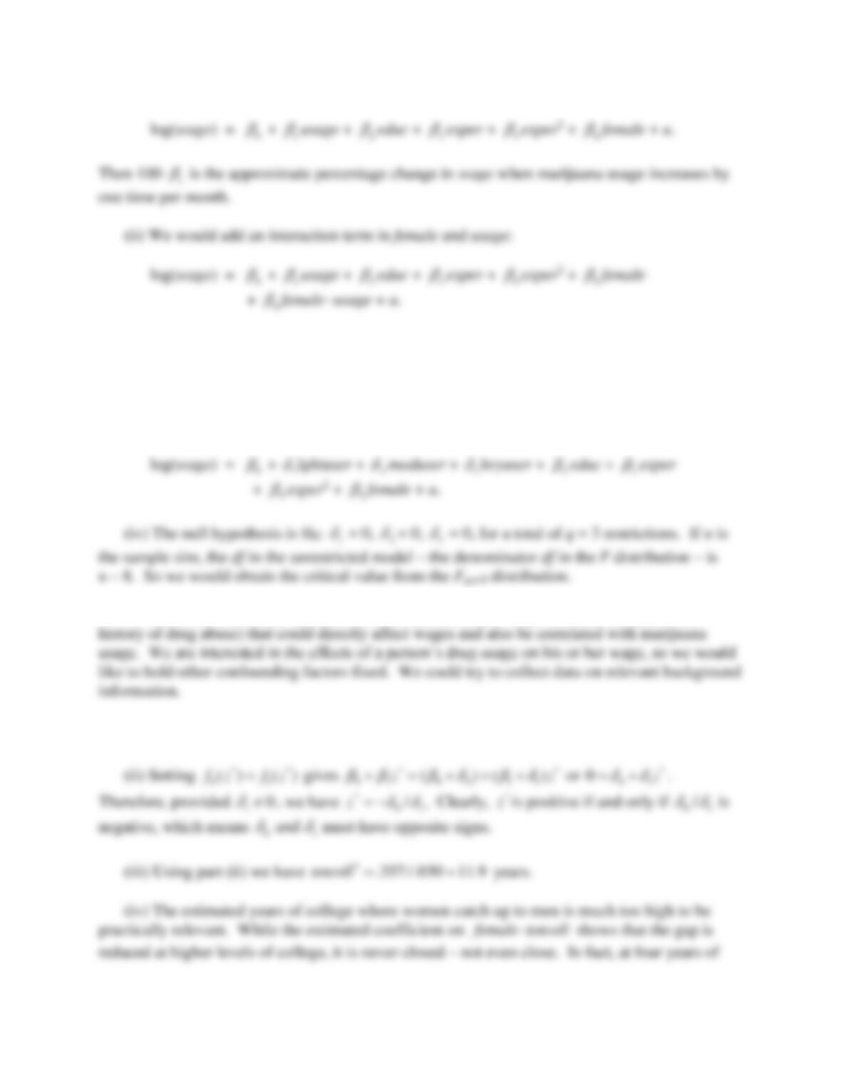
7.8 (i) We want to have a constant semi-elasticity model, so a standard wage equation with
marijuana usage included would be
75
The null hypothesis that the effect of marijuana usage does not differ by gender is H0:
6
= 0.
(iii) We take the base group to be nonuser. Then we need dummy variables for the other
three groups: lghtuser, moduser, and hvyuser. Assuming no interactive effect with gender, the
model would be
(v) The error term could contain factors, such as family background (including parental
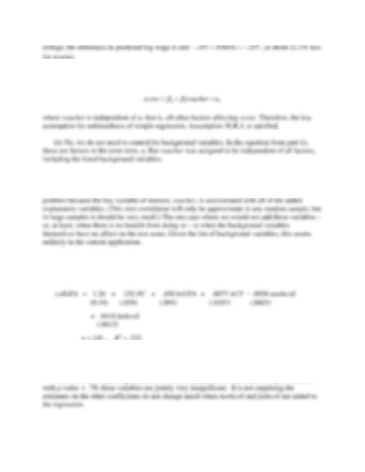
7.9 (i) Plugging in u = 0 and d = 1 gives
1 0 0 1 1
( ) ( ) ( )f z z
= + + +
.
76
7.10 (i) Yes, simple regression does produce an unbiased estimator of the effect of the voucher
program. Because participation was randomized, we can write
(iii) We should include the background variables to reduce the sampling error of the
estimated voucher effect. By pulling background variables out of the error term, we reduce the
error variance – perhaps substantially. Further, we can be sure that multicollinearity is not a
SOLUTIONS TO COMPUTER EXERCISES
C7.1 (i) The estimated equation is
n = 141 , R2 = .222.
The estimated effect of PC is hardly changed from equation (7.6), and it is still very significant,
with tpc
2.58.
(ii) The F test for joint significance of mothcoll and fathcoll, with 2 and 135 df, is about .24
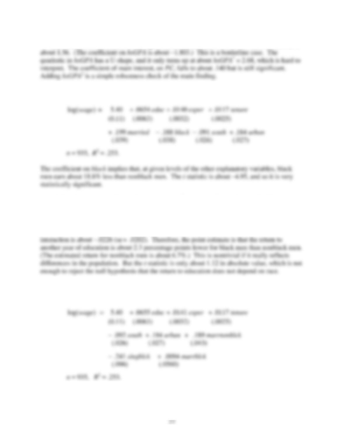
(iii) When hsGPA2 is added to the regression, its coefficient is about .337 and its t statistic is
C7.2 (i) The estimated equation is
(ii) The F statistic for joint significance of exper2 and tenure2, with 2 and 925 df, is about
1.49 with p-value
.226. Because the p-value is above .20, these quadratics are jointly
insignificant at the 20% level.
(iii) We add the interaction black
educ to the equation in part (i). The coefficient on the
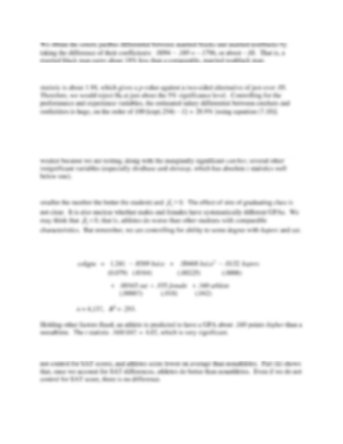
(iv) We choose the base group to be single, nonblack. Then we add dummy variables
marrnonblck, singblck, and marrblck for the other three groups. The result is
78
C7.3 (i) H0:
13
= 0. Using the data in MLB1.RAW gives
13
ˆ
.254, se(
13
ˆ
)
.131. The t
(ii) This is a joint null, H0:
9
= 0,
10
= 0, …,
13
= 0. The F statistic, with 5 and 339 df, is
about 1.78, and its p-value is about .117. Thus, we cannot reject H0 at the 10% level.
(iii) Parts (i) and (ii) are roughly consistent. The evidence against the joint null in part (ii) is
C7.4 (i) The two signs that are pretty clear are
3
< 0 (because hsperc is defined so that the
(ii) The estimated equation is
(iii) With sat dropped from the model, the coefficient on athlete becomes about .0054 (se
.0448), which is practically and statistically not different from zero. This happens because we do
79
(iv) To facilitate testing the hypothesis that there is no difference between women athletes
and women nonathletes, we should choose one of these as the base group. We choose female
nonathletes. The estimated equation is
(v) Whether we add the interaction female
sat to the equation in part (ii) or part (iv), the
C7.5 The estimated equation is
C7.6 (i) The estimated equation for men is
(ii) The F statistic (with 6 and 694 df) is about 2.12 with p-value
.05, and so we reject the
null that the sleep equations are the same at the 5% level.
(iii) If we leave the coefficient on male unspecified under H0, and test only the five
(iv) The outcome of the test in part (iii) shows that, once an intercept difference is allowed,
(ii) We can write the model underlying (7.18) as
(iii) The t statistic on female from part (ii) is about –8.17, which is very significant. This is
81
C7.8 (i) If the appropriate factors have been controlled for,
1
> 0 signals discrimination against
minorities: a white person has a greater chance of having a loan approved, other relevant factors
fixed.
(ii) The simple regression results are
(iii) When we add the other explanatory variables as controls, we obtain
1
ˆ
.129, se(
1
ˆ
)
6.45).
(iv) When we add the interaction white
obrat to the regression, its coefficient and t statistic
(v) The trick should be familiar by now. Replace white
obrat with white
(obrat – 32); the
coefficient on white is now the race differential when obrat = 32. We obtain about .113 and se
.020. So the 95% confidence interval is about .113 1.96(.020) or about .074 to .152. Clearly,
C7.9 (i) About .392, or 39.2%.
(ii) The estimated equation is
82
(iii) 401(k) eligibility clearly depends on income and age in part (ii). Each of the four terms
involving inc and age have very significant t statistics. On the other hand, once income and age
(iv) Somewhat surprisingly, out of 9,275 fitted values, none is outside the interval [0,1]. The
(vi) Of the 5,638 families actually ineligible for a 401(k) plan, about 81.7 are correctly
(vii) The overall percent correctly predicted is a weighted average of the two percentages
(viii) The estimated equation is
C7.10 (i) The estimated equation is
83
(ii) Including all three position dummy variables would be redundant, and result in the
dummy variable trap. Each player falls into one of the three categories, and the overall intercept
is the intercept for centers.
(v) Adding the terms
2
and marr exper marr exper
leads to complicated signs on the three
(vi) If in the regression from part (iv) we use assists as the dependent variable, the coefficient
C7.11 (i) The average is 19.072, the standard deviation is 63.964, the smallest value is –502.302,
and the largest value is 1,536.798. Remember, these are in thousands of dollars.
(ii) This can be easily done by regressing nettfa on e401k and doing a t test on
ˆe401k
; the
(iii) The equation estimated by OLS is
84
(iv) Only the interaction e401k(age − 41) is significant. Its coefficient is .654 (t = 4.98). It
(v) The effect of e401k in part (iii) is the same for all ages, 9.705. For the regression in part
(vi) I chose fsize1 as the base group. The estimated equation is
(vii) The SSR for the restricted model is from part (vi): SSRr = 30,215,207.5. The SSR for
signs on the income variables actually change across family size.)
C7.12 (i) For women, the fraction rated as having above average looks is about .33; for men, it is
(ii) The difference is about .04, that is, the percent rated as having above average looks is
85
(iii) The regression for men is
Using the standard approximation, a man with below average looks earns almost 20% less than a
man of average looks, and a woman with below average looks earns about 13.8% less than a
woman with average looks. (The more accurate estimates are about 18% and 12.9%,
(v) Given the number of added controls, with many of them very statistically significant, the
(vi) The SSR for women is 83.6933, for men it is 166.0841, and so the unrestricted SSR is
249.7774 (rounded to four decimal places). The SSR obtained by adding the dummy variable
86
C7.13 (i) 412/660 .624.
(ii) The OLS estimates of the LPM are
(iii) The F test, with 4 and 653 df, is 4.43, with p-value = .0015. Thus, based on the usual F
(iv) The model with log(faminc) fits the data slightly better: the R-squared increases to about
(v) The fitted probabilities range from about .185 to 1.051, so none are negative. There are
two fitted probabilities above 1, which is not a source of concern with 660 observations.
(vi) Using the standard prediction rule – predict one when
.5
i
ecobuy
and zero otherwise –
87
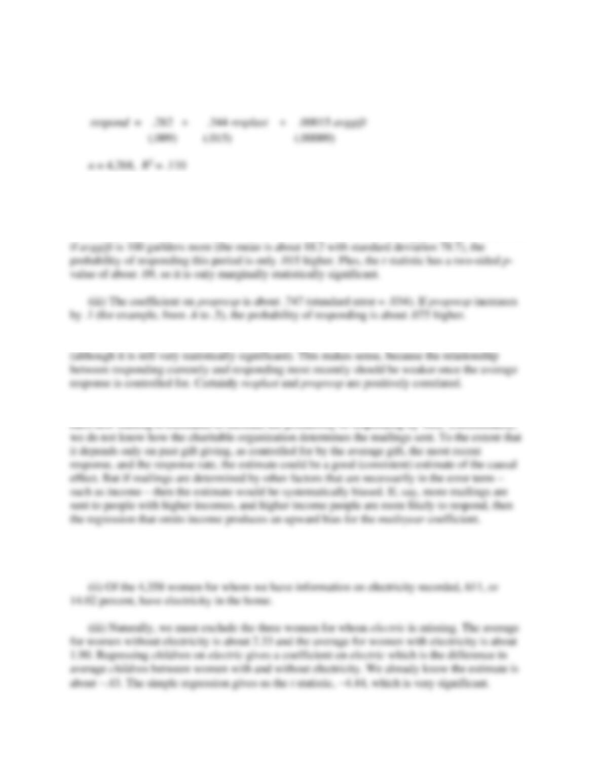
C7.14 (i) The estimated LPM is
Holding the average gift fixed, the probability of a current response is estimated to be .344
higher if the person responded most recently.
(ii) Once we control for responding most recently, the effect of of avggift is very small. Even
(iv) When propresp is added to the regression, the coefficient on resplast falls to about .095
(v) The coefficient on mailsyear is about .062 (t = 6.18). This is a reasonably large effect:
C7.15 (i) The smallest and largest values of children are 0 and 13. The average value is about
2.27. Naturally, no woman has 2.27 children.
88
(iv) We cannot infer causality because there can be many confounding factors that are
(vi) The coefficient on the interaction
electric educ
is −.022 and its t statistic is −1.31 (two-
(vii) If we use
( 7)electric educ−
instead, we force the coefficient on electric to be the effect