Chapter 7
Nonlinear, Semiparametric, and Nonparametric
Regression Models
◼ Exercises
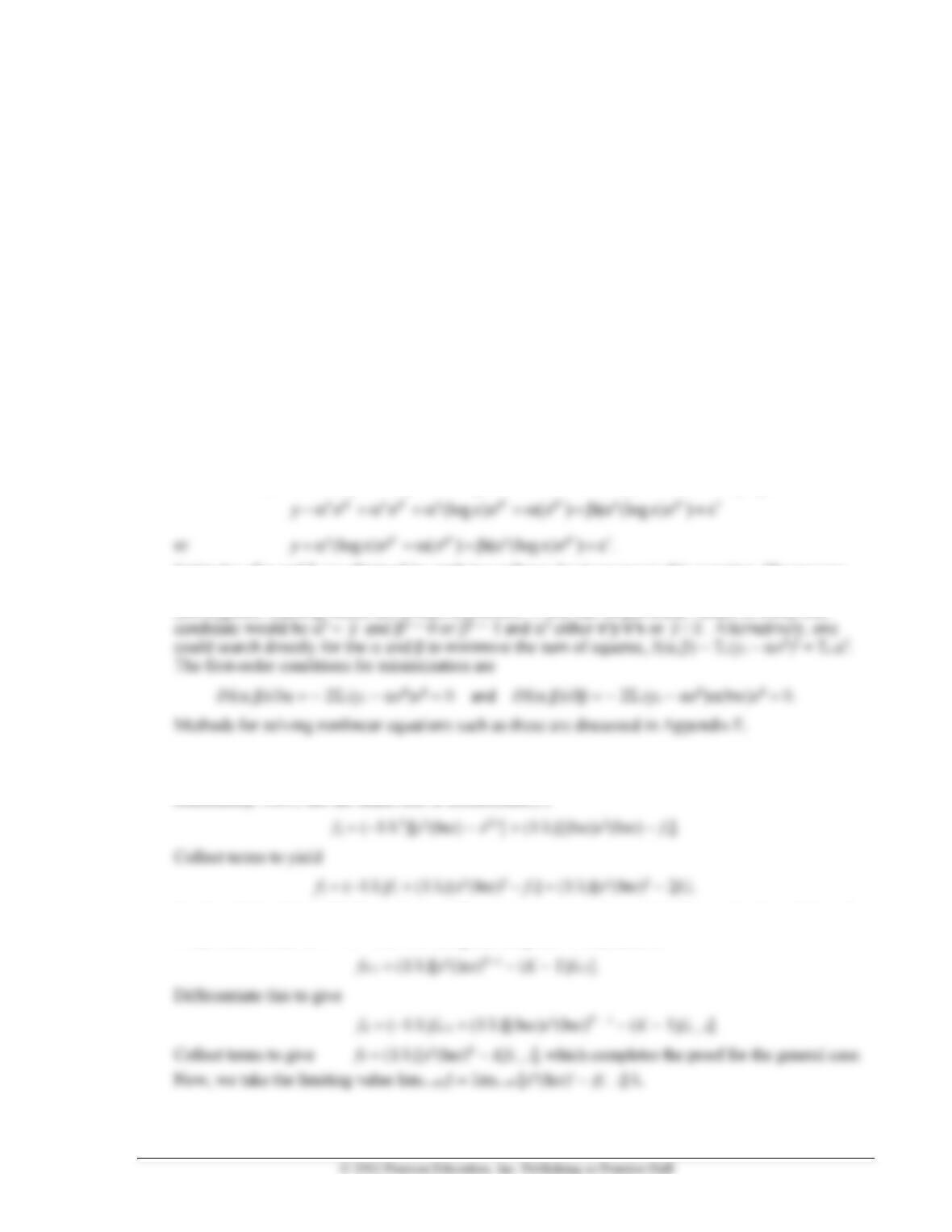
1. We cannot simply take logs of both sides of the equation as the disturbance is additive rather than
multiplicative. So, we must treat the model as a nonlinear regression. The linearized equation is
0 0 0
0 0 0 0
( ) (log ) ( )y x x x x
+ − + −
where 0 and 0 are the expansion point. For given values of 0 and 0, the estimating equation would be
Estimates of and are obtained by applying ordinary least squares to this equation. The process
is repeated with the new estimates in the role of 0 and 0. The iteration could be continued until
convergence. Starting values are always a problem. If one has no particular values in mind, one
2. The proof can be done by mathematical induction. For convenience, denote the ith derivative by fi.
The first derivative appears in Equation (7-34). Just by plugging in I = 1, it is clear that f1 satisfies the
relationship. Now, use the chain rule to differentiate f1,
So, the relationship holds for i = 0, 1, and 2. We now assume that it holds for i = K − 1, and show that
if so, it also holds for i = K. This will complete the proof. Thus, assume
50 Greene • Econometric Analysis, Seventh Edition
Use L’Hospital’s rule once again:
Applications
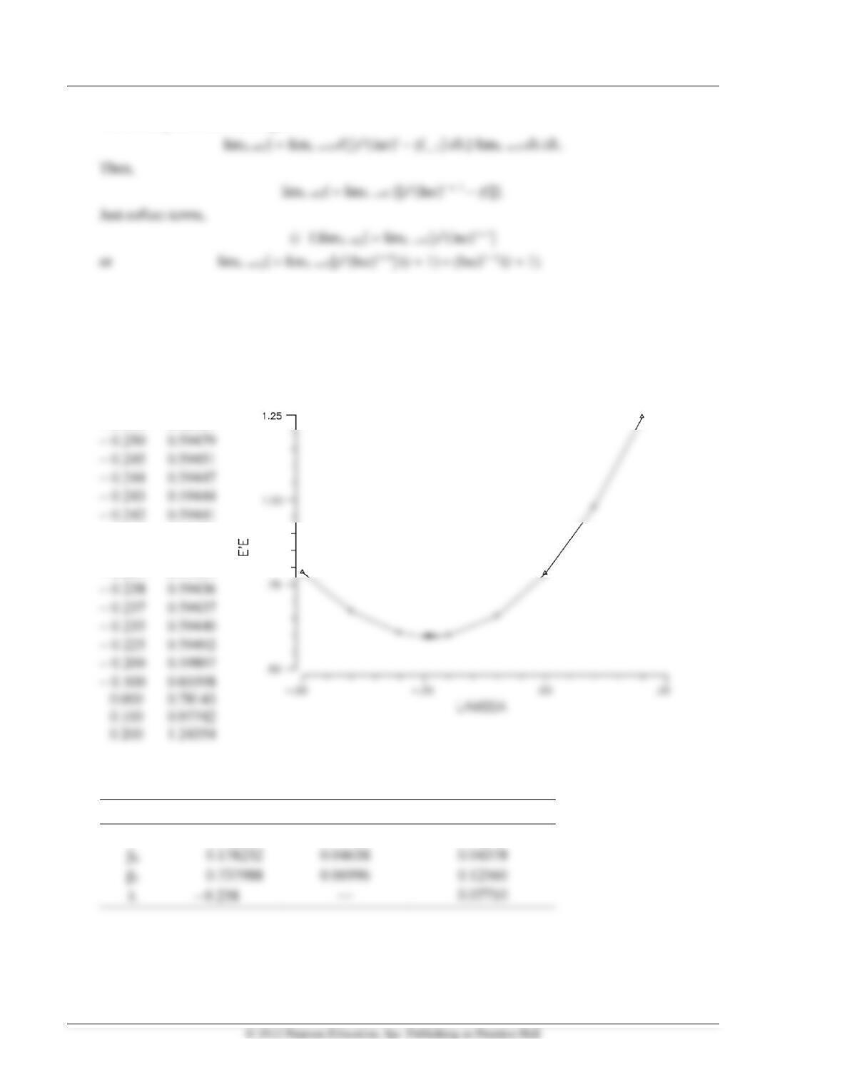
1. The search for the minimum sum of squares produced the following results:
ee
− 0.500 0.78477
− 0.400 0.67033
− 0.300 0.60587
− 0.241 0.59439
− 0.240 0.59438
− 0.239 0.59437
The sum of squared residuals is minimized at = −0.238. At this value, the regression results are as
follows:
Parameter
Estimate
OLS Std. Error
Correct Std. Error
2.06092
0.07718
0.09723
0.178232
0.04638
0.04378
Chapter 7 Nonlinear, Semiparametric, and Nonparametric Regression Models 51
Estimated Asymptotic Covariance Matrix
k
l
0.00945
k 0.00262
0.00192
l 0.00511
−0.00199
0.01578
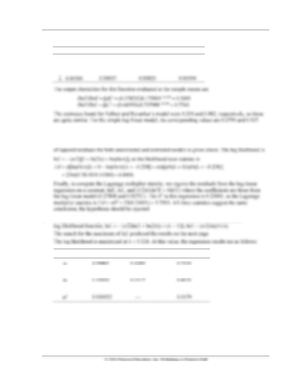
2. The Wald test is based on the unrestricted model. The statistic is the square of the usual t-ratio,
W = (− 0.232/0.0771)2 = 9.0546. The critical value from the chi-squared distribution is 3.84, so the
hypothesis that = 0 can be rejected. The likelihood ratio statistic is based on both models. The sum
3. Instead of minimizing the sum of squared deviations, we now maximize the concentrated
Parameter
Estimate
OLS Std. Error
Correct Std. Error
0.1283
0.7151
k
0.378094
0.1070
0.3228
l
0.1117
0.4121
0.124
—
0.2482
52 Greene • Econometric Analysis, Seventh Edition
Estimated Asymptotic Covariance Matrix
k
l
2
0.5114
k 0.2203
0.1042
0.0951
0.1698
0.1747
0.0730
0.0953
0.0617
0.0044
0.0059
0.0038
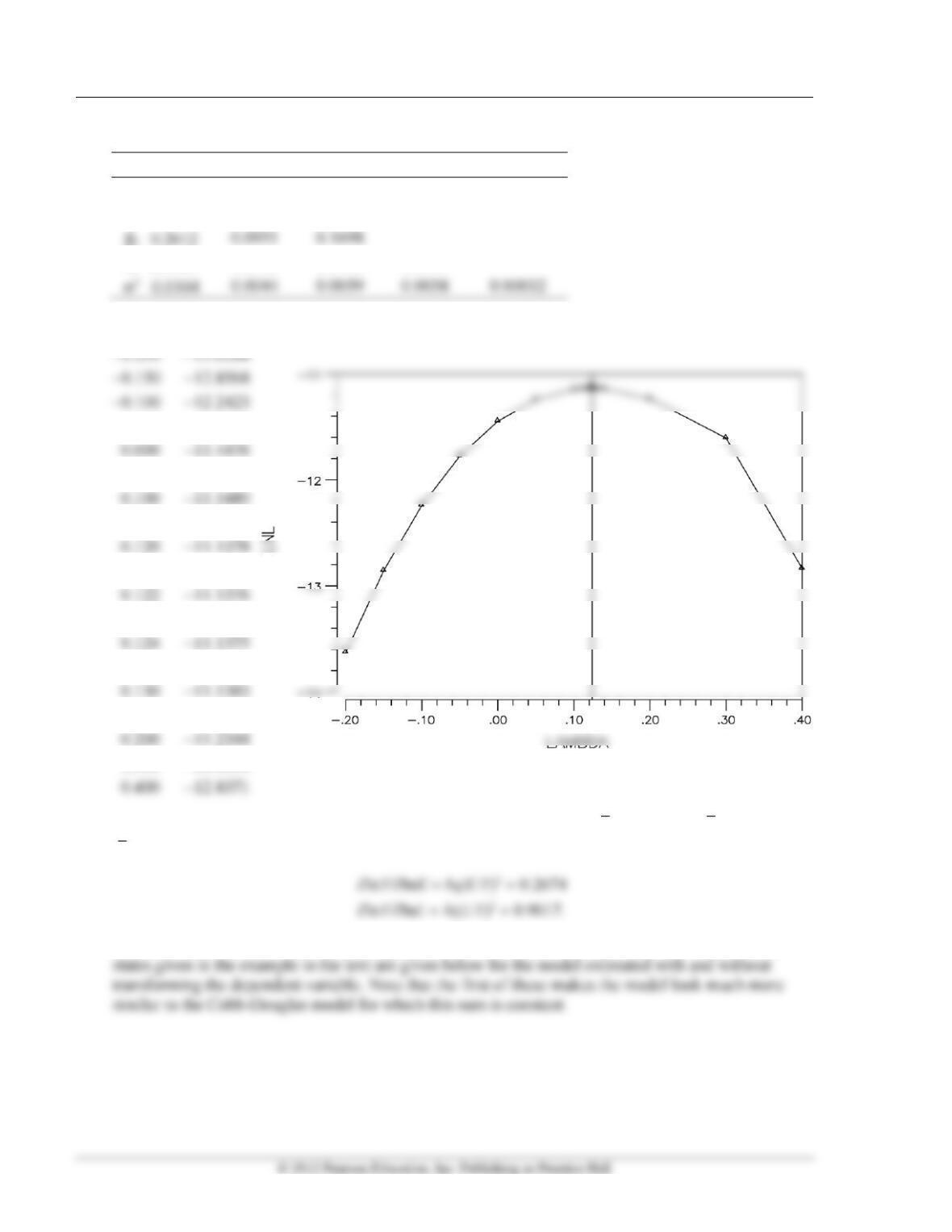
lnL
−0.050 −11.7764
0.050 −11.2427
0.110 −11.1410
0.121 −11.1377
0.123 −11.1376
0.125 −11.1376
0.140 −11.1423
0.300 −11.6064
The output elasticities for this function evaluated at the sample means,
0.175905,K=
0.737988,L=
2.870777,Y=
are
These are quite similar to the estimates given above. The sum of the two output elasticities for the
Chapter 7 Nonlinear, Semiparametric, and Nonparametric Regression Models 53
State
Full Box-Cox Model
lnQ on Left-Hand Side
Florida
1.2840
1.6598
Louisiana
1.2019
1.4239
California
1.1574
1.1176
Maryland
1.1657
1.0261
Ohio
1.1899
0.9080
Once again, we are interested in testing the hypothesis that = 0. The Wald test statistic is W = (0.123 /
0.2482)2 = 0.2455. We would now not reject the hypothesis that = 0. This is a surprising outcome.
The likelihood ratio statistic is based on both models. The sum of squared residuals for the restricted
4. This application actually does not work very well at all.
Sample ; 1 – 123 $
create ; wage=pl/1000$ <== the wage variable needed to be scaled for NLSQ.
Create ; k = cost*sk/pk ; m = cost*sl/wage $
—————————————————————————–
Ordinary least squares regression …………
LHS=LOGQ Mean = 8.17947
Residual Sum of Squares = 19.6402 119
——–+——————————————————————–
| Standard Prob. 95% Confidence
LOGQ| Coefficient Error t |t|>T* Interval
——–+——————————————————————–
54 Greene • Econometric Analysis, Seventh Edition
——–+——————————————————————–
Note: ***, **, * ==> Significance at 1%, 5%, 10% level.
—————————————————————————–
Cov.[b^]| ONE LOGK LOGM LOGKM
——–+——————————————————–
ONE| .145138 .151682 -.148244 .0765554
—————————————————————————–
WALD procedure. Estimates and standard errors
for nonlinear functions and joint test of
nonlinear restrictions.
——–+——————————————————————–
| Standard Prob. 95% Confidence
WaldFcns| Coefficient Error z |z|>Z* Interval
——–+——————————————————————–
GMA| 95197.9*** 36267.54 2.62 .0087 24114.9 166281.0
—————————————————————————–
calc ; c10=log(waldfns(1)) ? log gamma
; c20=waldfns(2) ? delta
; c30=waldfns(3) ? nu
; c40=waldfns(4) $ ? rho
nlsq ; lhs = logq
; labels = c1,c2,c3,c4
; fcn = c1 – (c3/c4)*log( c2/(k^c4) + (1-c2)/(m^c4))
; start = c10,.7,c30,c40 ? <== The estimate of delta was outside (0,1)
; output = 3;pri$
Itr 32 F= .9529D+01 gtHg= .1944D-01 chg.F= .2121D-02 max|db|= .5100D-02
1st derivs. .55004D-02 .20087D+02 -.20581D-01 -.90620D-03
Parameters: .11445D+02 .99989D+00 .11866D+01 -.33864D+01
Itr 33 F= .9528D+01 gtHg= .1164D-01 chg.F= .7744D-03 max|db|= .4248D-02
Itr 33 F= .9528D+01 gtHg= .2009D+02 chg.F= .1247D-06 max|db|= .2009D+02
Line search at iteration 33 does not improve fn. Exiting optimization.
Function= .78300061247D+02, at entry, .95279044765D+01 at exit
—————————————————————————–
User Defined Optimization…………………….
Nonlinear least squares regression …………
Chapter 7 Nonlinear, Semiparametric, and Nonparametric Regression Models 55
——–+——————————————————————–
| Standard Prob. 95% Confidence
UserFunc| Coefficient Error z |z|>Z* Interval
——–+——————————————————————–
C1| 11.4447*** .08192 139.71 .0000 11.2842 11.6053
—————————————————————————–
Cov.[b^]| C1 C2 C3 C4
——–+——————————————————–
C2| .216691E-04 .749667E-06 .315138E-05 -.00364865
5. Using the gasoline market data in Appendix Table F2.2, use the partially linear regression method in
Section 16.3.3 to fit an equation of the form
ln(G/Pop) =
1ln(Income) +
2lnPnew cars +
3lnPused cars + g(lnPgasoline) +
.
crea;gp=lg;ip=ly;ncp=lpnc;upp=lpuc;pgp=lpg$
sort;lhs=pgp;rhs=gp,ip,ncp,upp$
crea;dgp=.809*gp – .5*gp[-1] – .309*gp[-2]$
crea;dip=.809*ip – .5*ip[-1] – .309*ip[-2]$
crea;dnc=.809*ncp -.5*ncp[-1]-.309*ncp[-2]$
crea;duc=.809*upp -.5*upp[-1]-.309*upp[-2]$
samp;3-36$
regr;lhs=dgp;rhs=dip,dnc,duc;res=e$
+———————————————————————–+
| Ordinary least squares regression Weighting variable = none |
| Dep. var. = DGP Mean= .9708646870E-02, S.D.= .4738748109E-01 |
| Model size: Observations = 34, Parameters = 3, Deg.Fr.= 31 |
| Residuals: Sum of squares= .1485994289E-01, Std.Dev.= .02189 |
+———————————————————————–+
+———+————–+—————-+——–+———+———-+
|Variable | Coefficient | Standard Error |t-ratio |P[|T|>t] | Mean of X|
+———+————–+—————-+——–+———+———-+
+—————————————————+
|Number of observations in current sample = 34 |
56 Greene • Econometric Analysis, Seventh Edition
+———+————–+—————-+——–+———+
|Variable | Coefficient | Standard Error |b/St.Er.|P[|Z|>z] |
+———+————–+—————-+——–+———+
B_1 .9629902959 .13004843 7.405 .0000
6.
+—————————————+
| Nonparametric Regression for G |
| Observations = 36 |
| Points plotted = 36 |
| Bandwidth = .468092 |
| Statistics for abscissa values—- |
| Mean = 2.316611 |