CHAPTER 7
Economic Growth: Malthus and Solow
KEY IDEAS IN THIS CHAPTER
1. There are eight primary facts of economic growth that are key to organizing our
thinking about economic growth.
2. In the Malthusian model of economic growth, population growth increases with the
3. The Malthusian model does a good job of explaining economic growth prior to the
4. Unlike the Malthusian model, capital accumulation plays an important role in the
Solow growth model.
5. The Solow growth model predicts that long-run improvements in the standard of
7. Growth accounting is an approach to decomposing economic growth to factor input
growth and total factor productivity growth.
NEW IN THE THIRD EDITION
1. New: “Theory Confronts the Data: The Recent Trend in Economic Growth in
Canada”
3. Charts and tables have been updated to reflect new data.
4. End-of-chapter problems have been added.
Chapter 7: Economic Growth: Malthus and Solow
TEACHING GOALS
Students easily take for granted the much more abundant standard of living of today as
opposed to twenty, fifty, or one hundred years ago. Sometimes it is easier to remind
students of what their ancestors had to do without, rather than simply referring to per
capita income levels over time. Recessions come and go, and yet economic growth
swamps the lost output we endure during hard times. The most recent recession is unlike
the Great Depression, in that the drop in GDP below trend is not as large and is not as
prolonged, and our times are certainly not at all like the Great Depression in that our
incomes are many times larger than those of the typical person in Canada in the 1930s.
The typical student begins the study of economic growth against the backdrop of the
recent growth experience of Canada. The current standard of living in Canada vastly
surpasses the current standard of living in most countries and would have been
unimaginable anywhere in the world before the advent of the Industrial Revolution. Until
CLASSROOM DISCUSSION TOPICS
Getting students to relate to differences in standards of living can sometimes be difficult.
It is easy to take one’s own standard of living for granted. An interesting discussion topic
is whether students would be willing to travel back in time to 100 or 200 years ago, if
they could be one of the richest people of those earlier times. Would the trade-off be
worthwhile? While students typically stress factors like antiquated views about freedom
of choice and racial and gender issues, try to encourage students to direct their concerns
to those that are more economic than social. Also point out that higher standards of living
allow societies to be more concerned about issues of equality when mere survival is no
longer precarious.
Instructor’s Manual for Macroeconomics, Fourth Canadian Edition
Students often view population growth as the result of cultural factors and personal
preferences. Against the abundance of daily living, it is easy to forget economic factors.
Ask the students for examples of economic factors that might influence fertility decisions.
The Malthusian model suggests that growth may only be achieved through population
control. In the modern economy, the costs of raising children can be formidable, and so
there is a tendency for such costs to be a disincentive to fertility. Such costs may
contribute to the tendency for low fertility rates in advanced economies. In less developed
societies, having a large family can be a private form of social security. The more
children a family has, the more children there will be to provide for the parents in old age.
Poor public health conditions may actually enhance fertility. If each child has a smaller
chance for survival to adulthood, more births are required to produce a given-sized
family.
A major goal of most countries is to have sustained growth in per capita real GDP. Ask
students whether this is an appropriate goal for all countries in all periods. Is growth
always beneficial? What problems can growth bring?
Although growth normally leads to more jobs and a greater availability of goods and
OUTLINE
1. Economic Growth Facts
a) Pre-1800: Constant per Capita Income across Time and Space
b) Post-1800: Sustained Growth in the Rich Countries
2. The Malthusian Model
a) Production Determined by Labour and Fixed Land Supply
b) Population Growth and per Capita Consumption
c) Steady-State Consumption and Population
i) Effects of Technological Change
ii) Effects of Population Control
d) Malthus: Theory and Evidence
3. Solow’s Model of Exogenous Growth
a) The Representative Consumer
b) The Representative Firm
c) Competitive Equilibrium
d) Steady-State Growth
f) Labour Force Growth and Output per Worker
g) Total Factor Productivity and Output per Worker
4. Growth Accounting
a) Solow Residuals
b) The Productivity Slowdown
i) Measurement of Services
ii) The Relative Price of Energy
TEXTBOOK QUESTION SOLUTIONS
Problems
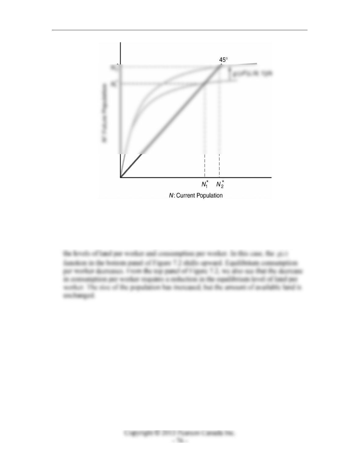
1. The amount of land increases and, at first, the size of the population is unchanged.
Therefore, consumption per worker increases. However, the increase in consumption
per worker increases the population growth rate. In the steady state, neither *
c nor *
l
are affected by the initial increase in land. This fact can be discerned by noting that
there will be no changes in either of the panels of Figure 6.8 in the textbook. (This
figure is also reproduced as Figure 7.1, below.)
Instructor’s Manual for Macroeconomics, Fourth Canadian Edition
Figure 7.1
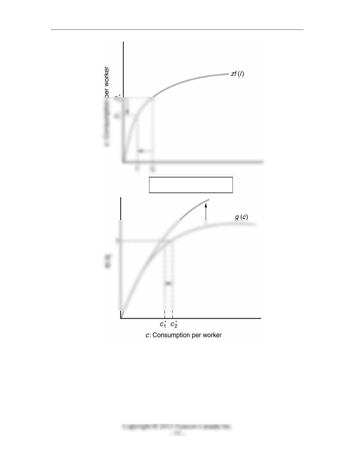
2. A reduction in the death rate increases the number of survivors from the current
period who will still be living in the future. Therefore, such a technological change in
public health shifts the function ()
g
c upward. In Problem 1 there were no effects on
g
Chapter 7: Economic Growth: Malthus and Solow
Figure 7.2
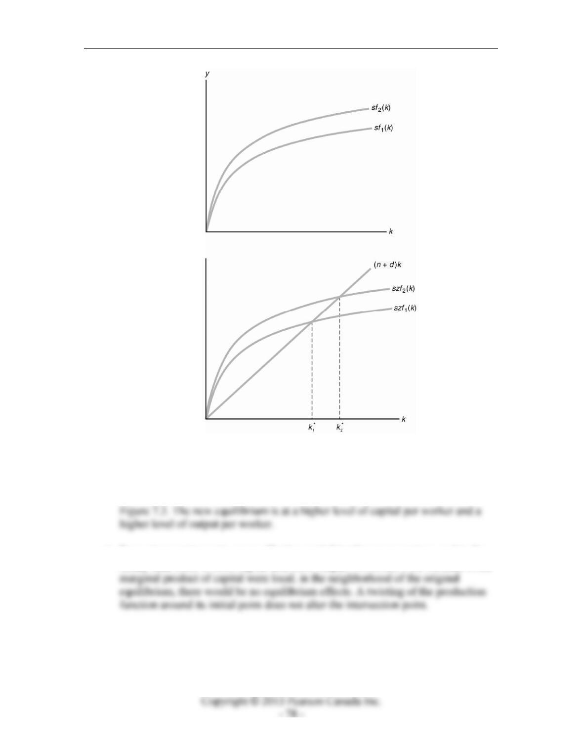
3. For the marginal product of capital to increase at every level of capital, the shift in the
production function is equivalent to an increase in total factor productivity.
a) The original and new production functions are shown in Figure 7.3 below.
l : Land per worker
Instructor’s Manual for Macroeconomics, Fourth Canadian Edition
Figure 7.3
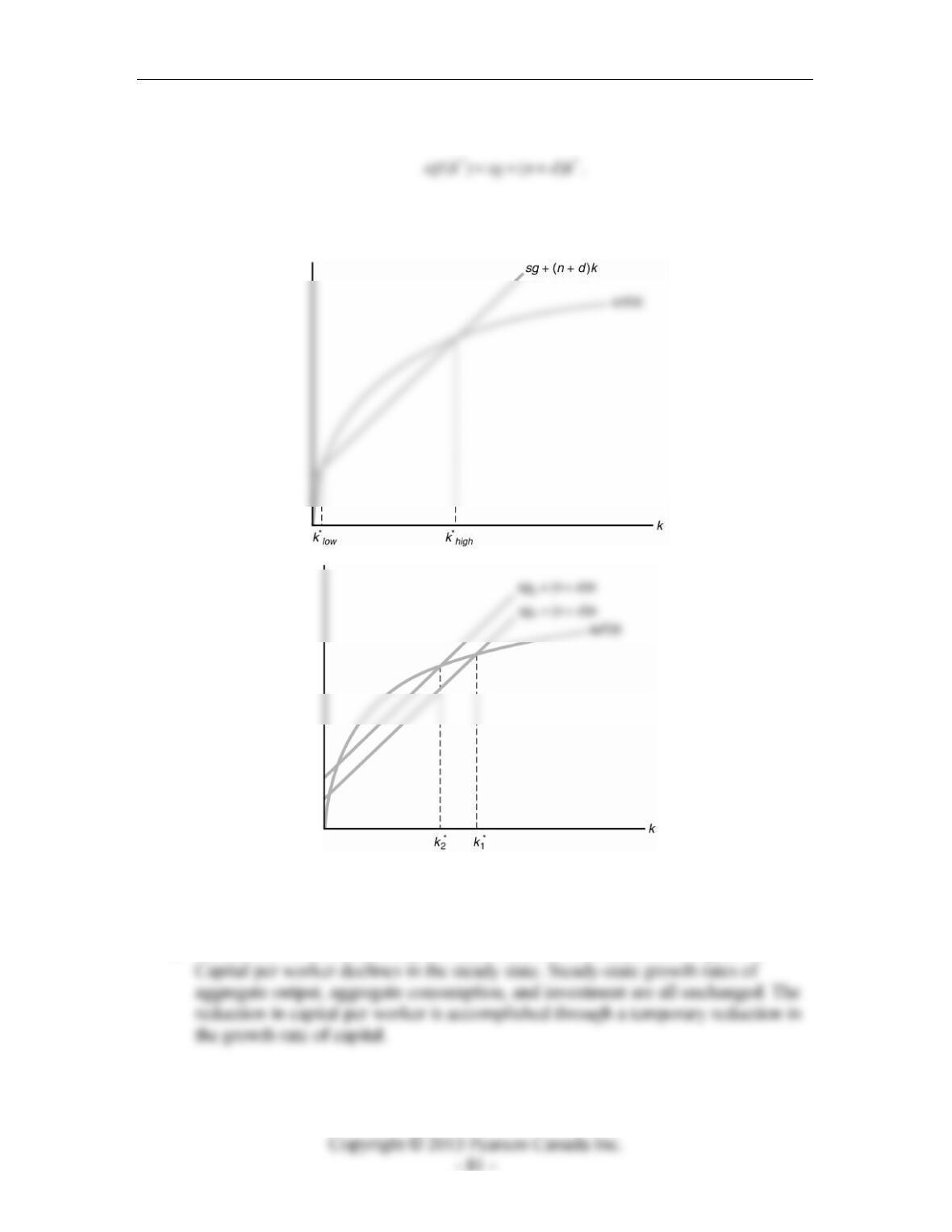
b) Equilibrium in the Solow model is at the intersection of ()
s
zf k with the line
segment ()ndk+. The old and new equilibria are depicted in the bottom panel of
c) For a given savings rate, more effective capital implies more savings, and in the
steady state there is more capital and more output. However, if the increase in the
4. An increase in the depreciation rate acts in much the same way as an increase in the
population growth rate. More of current savings is required just to keep the amount of
capital per worker constant. In equilibrium, output per worker and capital per worker
decrease.
5. Destruction of capital.
a) The long-run equilibrium is not changed by an alteration of the initial conditions.
If the economy started in a steady state, the economy will return to the same
steady state. If the economy were initially below the steady state, the approach to
the steady state will be delayed by the loss of capital.
the likely adjustment to a loss of capital.
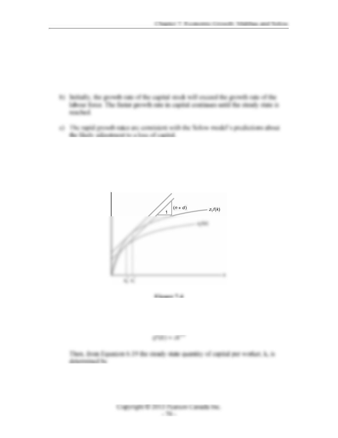
6. A reduction in total factor productivity reduces the marginal product of capital. The
Golden Rule level of capital per worker equates the marginal product of capital with
nd+. Therefore, for given nd+, the Golden Rule amount of capital per worker must
decrease as in Figure 7.4, below. Therefore the Golden Rule savings rate must
decrease.
Figure 7.4
7. a) Given the production function, we can write the per-worker production function
as
,11.02.0 5.0 kk =
Instructor’s Manual for Macroeconomics, Fourth Canadian Edition
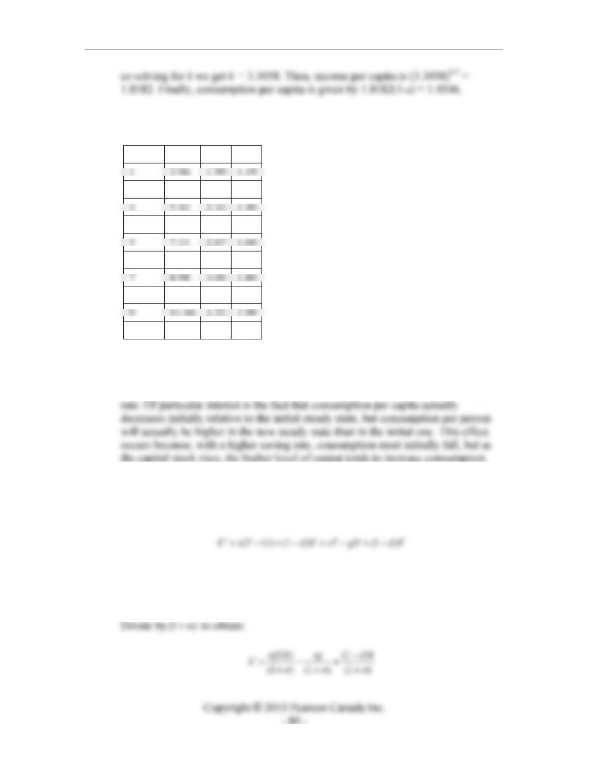
b) 1.4545 1.1939 1.2964 1.3982 1.4994 1.5998 1.6995 1.7985 1.8966
1.9939 2.0905
Period k y c
2 4.67 2.16 1.30
4 6.25 2.50 1.50
6 8.02 2.83 1.70
8 9.99 3.16 1.90
10 12.14 3.48 2.09
In the new steady state, with s = 0.4, calculating the steady state as before, we get
k = 13.22, y = 3.64, and c = 2.18. Note that after 10 periods, the economy is much
closer to the new steady state than to the old steady state with the lower savings
8. Government spending in the Solow model.
a) By assumption, we know that T = G, and so we may write:
Now divide by N and rearrange as:
‘(1 ) ( ) (1 )knszfksg dk+= −+−
Chapter 7: Economic Growth: Malthus and Solow
Setting k = k’ we find that:
s
This equilibrium condition is depicted in Figure 6.5.
Figure 7.5
b) The two steady states are also depicted in Figure 7.5.
c) The effects of an increase in g are depicted in the bottom panel of Figure 7.5.
9. The Golden Rule quantity of capital per worker *
k is such that *
()
K
M
Pzfk nd
′
==+. A
decrease in the population growth rate, n, requires a decrease in the marginal product
Instructor’s Manual for Macroeconomics, Fourth Canadian Edition
10. a) Capital evolves over time, as in Equation 7.16, according to
KdbNKszFK )1(),(‘ −+= .
Now, simplifying, as for Equation 7.17, we get
11. Production linear in capital:
() ()
YK
zzfkfkk
NN
== =.
a) Recall Equation 6.18 from the textbook, and replace ()
f
k with k to obtain:
((1)
‘(1 )
s
zd
kk
n
+−
=
+.
N
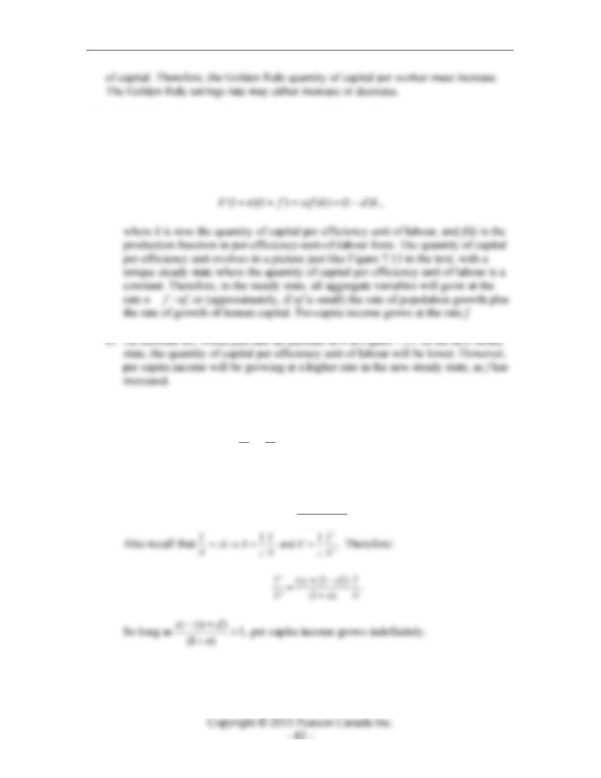
b) The growth rate of income per capita is therefore:
Chapter 7: Economic Growth: Malthus and Solow
‘
((1))
‘1
(1 )
YY
sz d
NN
gYn
−+−
== −
+
c) This model allows for the possibility of an ever-increasing amount of capital per
capital per worker.
12. For convenience, normalize by setting N = 1, so that per capita variables are the
same as levels. First, calculating the steady state capital stock when z=1, from equation
(7.19),
**
()( )szf k n d k=+ ,
So plugging in for f(k) and the parameters assumed in this problem, we have
Further, savings is equal to investment, or
*0.27savings investment sy===
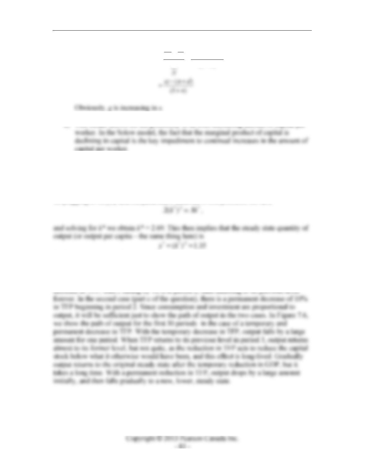
We then start the economy in the first period in this steady state, and consider two
alternative scenarios. In the first (part b of the question), we consider a temporary
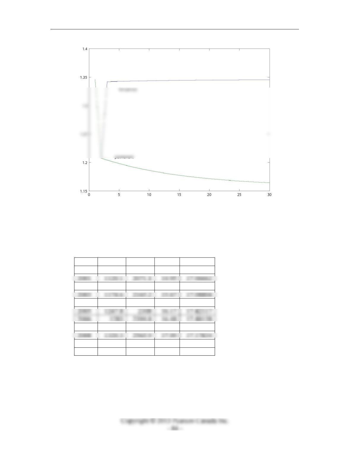
Instructor’s Manual for Macroeconomics, Fourth Canadian Edition
Figure 7.6
13. Solow residual calculations.
a)
Year Y K N z
2000 1100.5 2026.1 14.76 17.03065
2002 1152.9 2113.6 15.31 17.17126
2004 1211.2 2229.7 15.95 17.25081
2007 1311.3 2479.5 16.87 17.39451
2009 1283.7 2607.6 16.81 16.81488
2010 1325 2668.7 17.04 17.0725

Chapter 7: Economic Growth: Malthus and Solow
b) Percentage Growth Rates
Year Y K N z
2001 1.781009 2.221016 1.287263 0.21121
2003 1.88221 2.441332 2.351404 -0.48464
2005 3.021797 3.511683 1.37931 0.987536
2007 2.205768 3.53683 2.366505 -0.49694
2010 3.217263 2.343151 1.368233 1.532105
From year to year, note that growth in the capital stock is least variable, growth in