Economics Chapter 7 Homework Both Models Give Similar Results One Advantage

Basic Econometrics, Gujarati and Porter

61

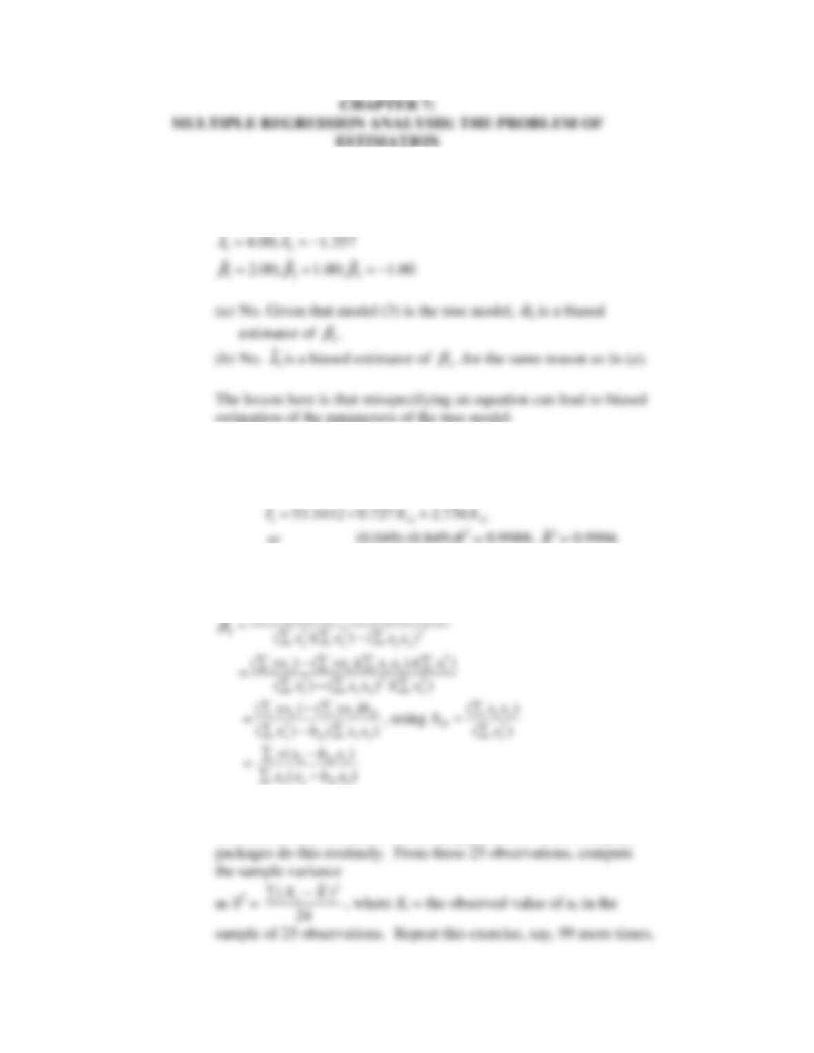
7.1 The regression results are:

1 2

ˆ ˆ

3.00; 3.50

α α

= − =

7.2 Using the formulas given in the text, the regression results are as

follows:

7.3 Omitting the observation subscript i for convenience, recall that

2

( )( ) ( )( )

yx x yx x x

∑ ∑ −∑ ∑

7.4

Since we are told that is, u

i

~ N(0,4), generate, say, 25 observations

from a normal distribution with these parameters. Most computer

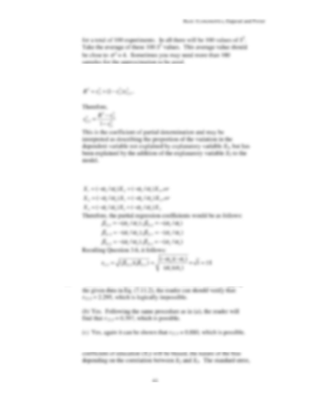
7.5

From Eq. (7.11.7) from the text, we have

7.6

The given equation can be written as:

7.7

(a) No. An r-value cannot exceed 1 in absolute value. Plugging

7.8

If you leave out the years of experience (X

3

) from the model, the

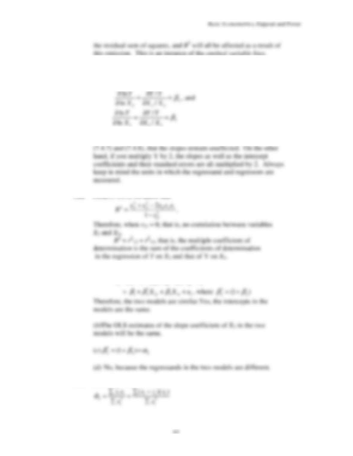
7.9

The slope coefficients in the double-log models give direct estimates

of the (constant) elasticity of the left-hand side variable with respect

to the right hand side variable. Here:

7.10

(a) & (b) If you multiply X

2

by 2, you can verify from Equations

7.12

(a) Rewrite Model B as:

(1 )

Y X X u

β β β

= + + + +

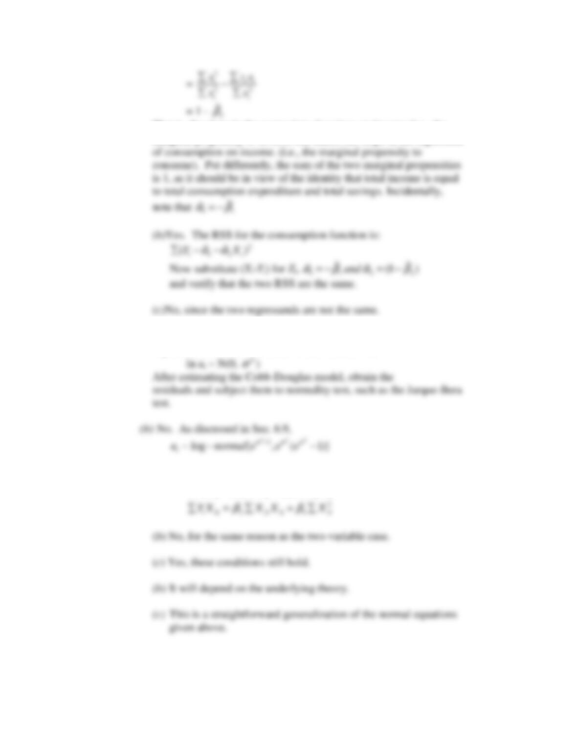
7.13

(a) Using OLS, we obtain:

Basic Econometrics, Gujarati and Porter

64

That is, the slope in the regression of savings on income (i.e., the

marginal propensity to save) is one minus the slope in the regression

7.14

(a) As discussed in Sec. 6.9, to use the classical normal linear

regression model (CNLRM), we must assume that

7.15

(a) The normal equations would be:

2

2 2 2 3 2 3

i i i i i

Y X X X X

β β

∑=∑+∑

Basic Econometrics, Gujarati and Porter

65

Empirical Exercises

7.16

(a)

Linear Model:

( b)

Log-Linear Model

2 3 4 5

ˆ

ln 0.627 1.274ln 0.937 ln 1.713ln 0.182 ln

t i i i i

Y X X X X

= − + + −

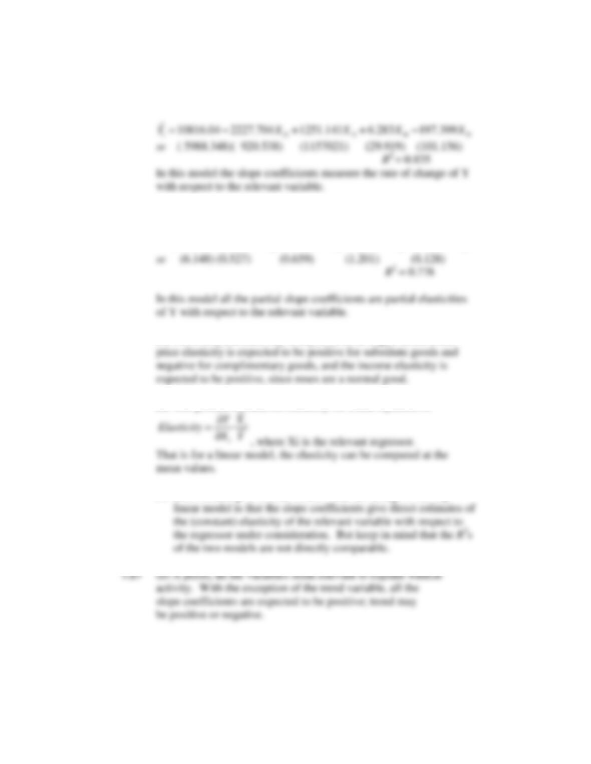
(c) The own-price elasticity is expected to be negative, the cross

(d)

The general formula for elasticity for linear equation is:

(e)

Both models give similar results. One advantage of the log-

(b) The estimated model is:

2 3 4 5

ˆ

37.186 2.775 24.152 0.011 0.213

i i i i i

Y X X X X

= − + + − −

se = ( 12.877) (0.57) ( 5.587) (0.008) (0.259)

Basic Econometrics, Gujarati and Porter

66

(c)

Price per barrel and domestic output variables are statistically

(d)

The log-linear model may be another specification. Besides

7.18

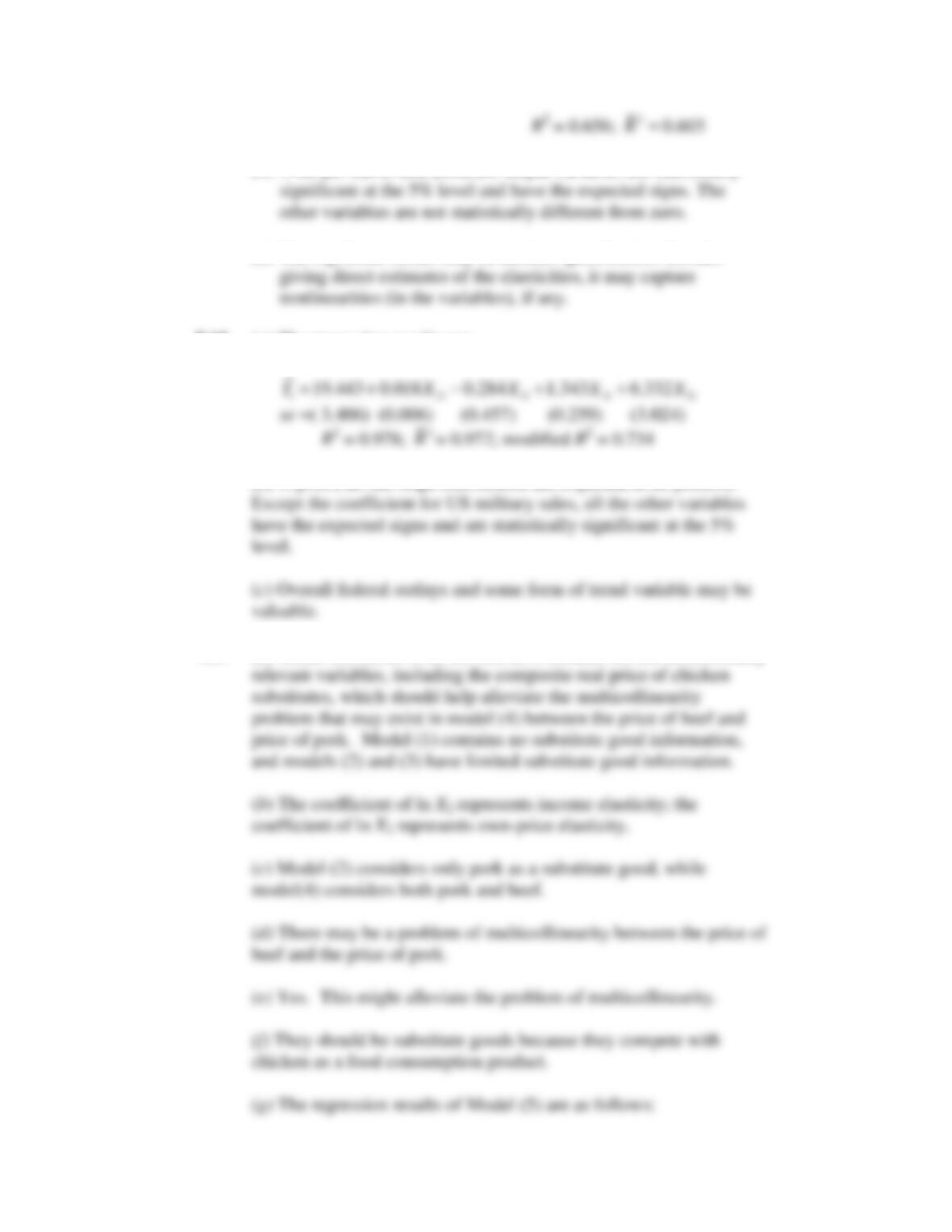
(a) The regression results are:

(b) A priori, all the slope coefficients are expected to be positive.

7.19

(a) Model (5) seems to be the best as it includes all the economically

(h) The consequence of estimating model (2) would be that the

7.20

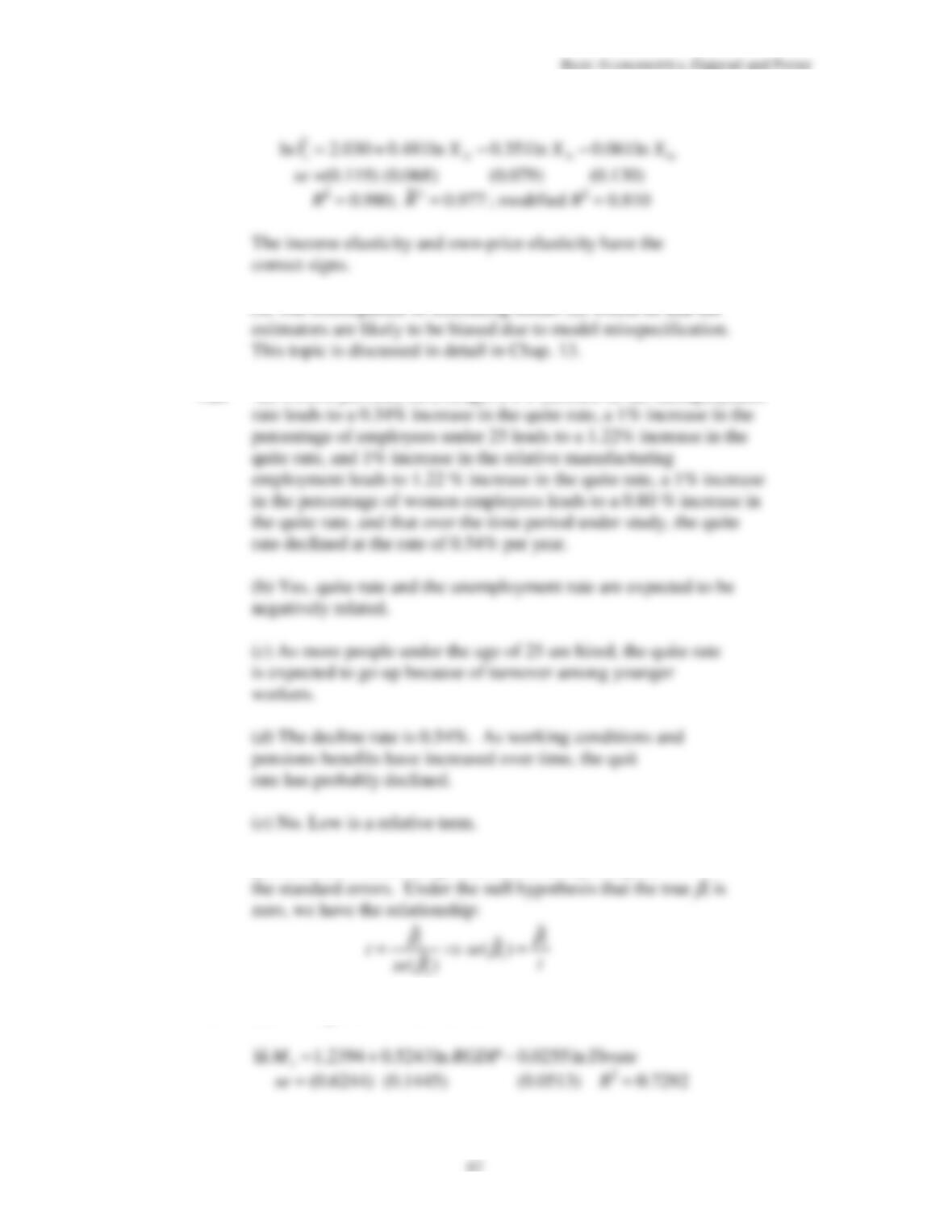
(a) Ceteris paribus, on average, a 1% increase in the unemployment

(f) Since the t values are given, we can easily compute

7.21

(a) The regression results are as follows:

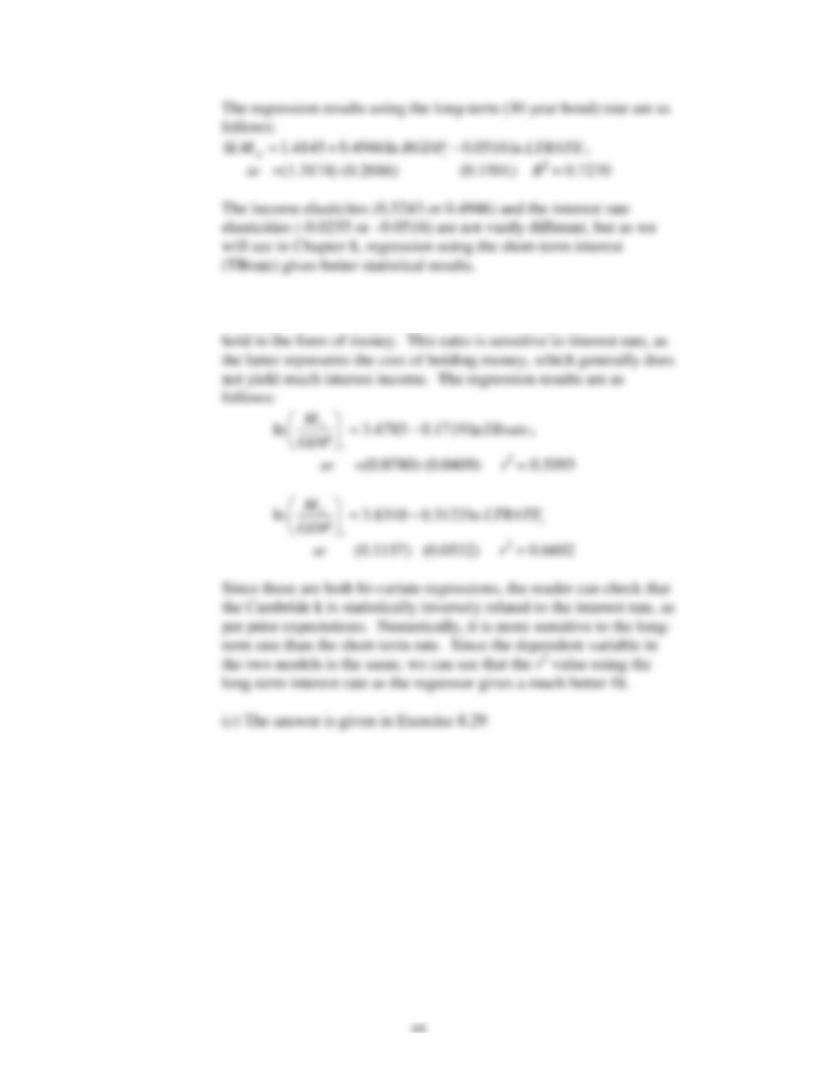
Basic Econometrics, Gujarati and Porter

(b) The ratio, M/GDP is known in the literature as the

Cambridge

k.

It represents the proportion of the income that people wish to

7.22

The results of fitting the Cobb-Douglas production function,

obtained from EViews3 are as follows:

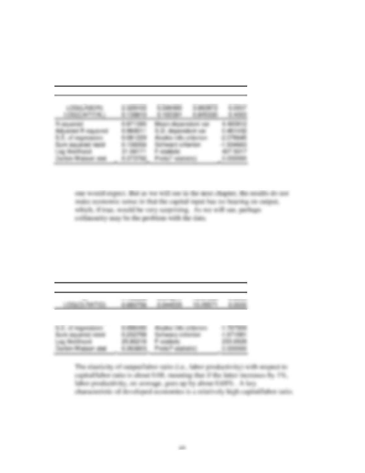
Basic Econometrics, Gujarati and Porter

Dependent Variable: LOG(OUTPUT)

.

Sample: 1961 1987

Included observations: 27

Variable Coefficient

Std. Error

t-Statistic

Prob.

C -11.93660

3.211064

-3.717335

0.0011

(a) The estimated output/labor and output/capital elasticities are positive, as

(b)

The regression results are as follows:

Dependent Variable: LOG(PRODUCTIVITY)

.

Sample: 1961 1987

Included observations: 27

Variable Coefficient

Std. Error

t-Statistic

Prob.

R-squared 0.903345

Mean dependent var –2.254332

Adjusted R-squared 0.899479

S.D. dependent var 0.304336

70

7.23

This is a class exercise. Note that your answer will depend on the

7.24

(a)

(b) The three independent variables are statistically significant at the

7.25

(a) Using a transformed time index (where t = 1 for the first

observation on 1/3/95 and t = 260 on 12/20/99), the linear regression

model is:

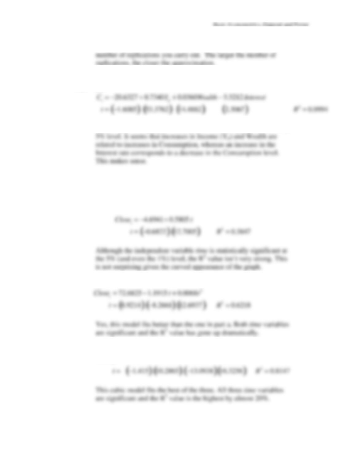
(b)

(c)

Close

t

= −10.8543 +2.6128 t−0.0296t

2

+0.00009t

3