1
CHAPTER 7
Costs
A. Summary
This chapter defines input costs and relates these cost concepts to the produc-
tion function. In the initial section on definitions, some care is taken to dis-
tinguish between economic and accounting costs and to show why economic
concepts are more appropriate for theoretical investigations. The concept of
opportunity cost for the firm is stressed throughout this discussion.
The bulk of the chapter concerns the relationship between input costs and
the production function. The firm’s expansion path is introduced to show that
B. Lecture and Discussion Suggestions
There seems no ready escape from a flood of cost curves when lecturing on
this chapter. The curves are both important and relatively difficult to derive
so it is probably impossible to avoid repeating the text to some degree. Over
the years we have shortened the material on differences between the short
and long runs, and we believe the profession has been moving that way, too
(especially in the theory of industrial organization). For lectures, therefore,
we would suggest focusing on long-run average and marginal cost concepts
Chapter 7: Costs
2
C. Modeling the Short and Long Run
The textbook model of fixed costs in the short run is a very standard one used
in the profession. Still, there are some apparent inconsistencies among defi-
nitions that can be resolved if the model is thought about in the right way.
The textbook says that fixed costs equal expenditures 𝑣𝐾1 on capital 𝐾1
that cannot be adjusted in the short run. But isn’t 𝑣𝐾1 a sunk cost which
know it exactly.
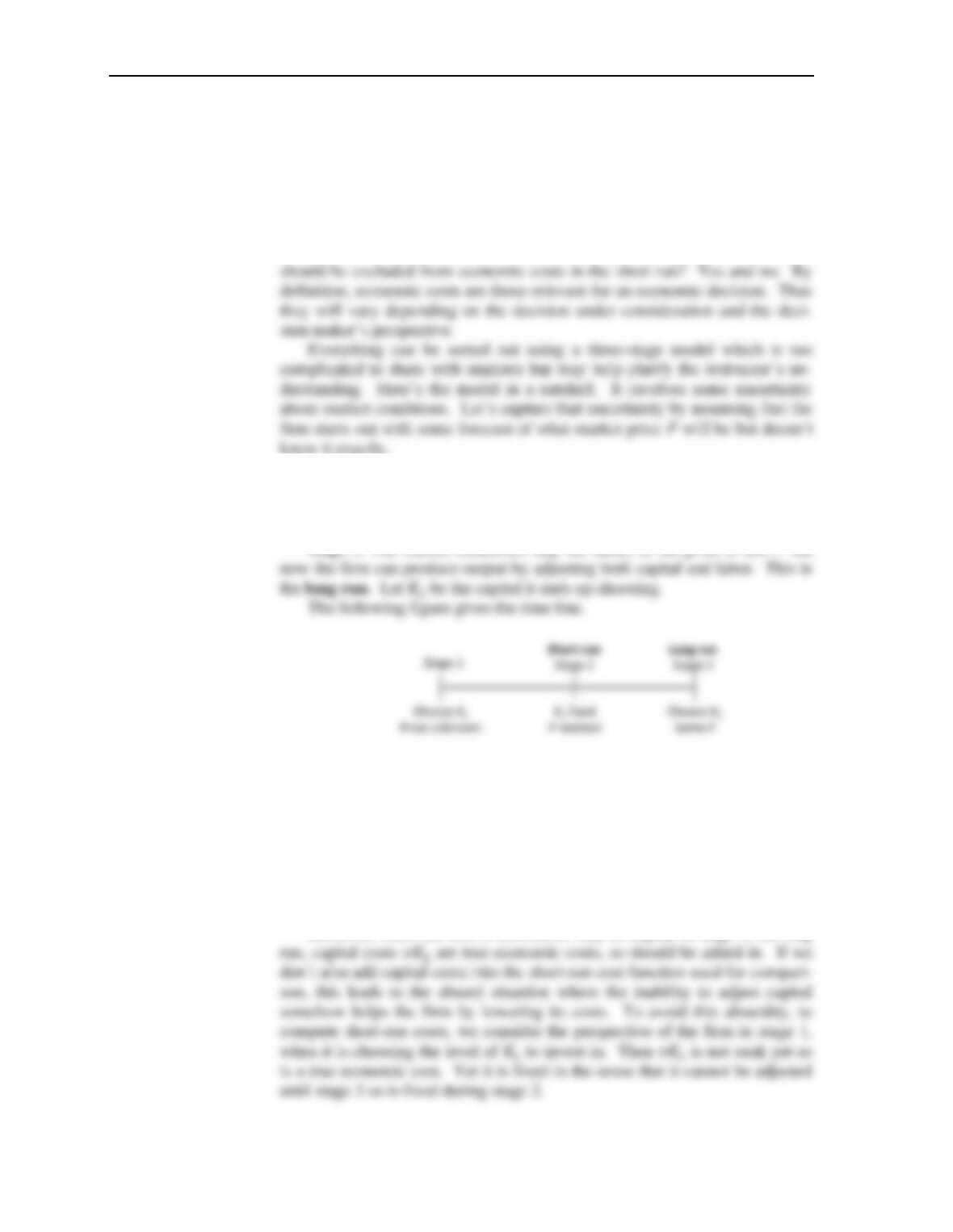
Stage 1: The firm builds capacity 𝐾1.
Stage 2: The firm learns the market price 𝑃. It chooses output to maxim-
ize profits knowing 𝑃. It is free to adjust labor but must stick with capital 𝐾1.
This is the short run.
Stage 3: The market conditions stay the same, so the price is still 𝑃 but
If we put the firm in stage 2 and look at its shut-down decision having al-
ready invested in its capital, then 𝑣𝐾1 is indeed sunk and should not factor
into economic costs going forward. This is exactly why the firm compares
revenue from continued operation only to variable costs in Chapter 8; if vari-
able costs can be covered, the firm should operate; if not the firm should shut
down. The firm may end up operating even if it can’t also cover 𝑣𝐾1 be-
cause that, being sunk, is an accounting but not a true economic cost at that
point.
However, when the firm is allowed to vary its capital in stage 3, the long
Chapter 7: Costs
3
It isn’t important to keep this complicated structure in mind but it should
at least provide some comfort that all the definitions can, with some effort, be
made consistent with each other. It also reinforces the point that economic
cost is a relativistic concept, depending on who the decision maker is (indi-
vidual? firm? social planner?) as well as which decision it is making (matric-
ulating in college or dropping out? firm output or entry?).
D. Returns to Scale vs. Economies of Scale
The new edition introduces the definitions of economies and diseconomies of
scale. Previous editions just talked about returns to scale. The two sets of
concepts are related. For certain classes of production functions they are
synonymous. For example, a production function that is everywhere increas-
ing returns to scale will have a downward sloping AC curve, thus exhibiting
E. Glossary Entries in the Chapter
• Accounting Costs
• Average Cost
• Depreciation Schedule
• Economic Costs
• Economic Profits (𝜋)
• Economies of Scope
Chapter 7: Costs
4
SOLUTIONS TO CHAPTER 7 PROBLEMS
7.1 a.
b. Since RTS = 1/2 < w/v = 1, the manufacturer will use only K. For q = 20, K =
7.2 a. Because the manufacturer does not change its input mix in response to chang-
ing input prices, the cost of producing 1,000 gumballs will always be the cost
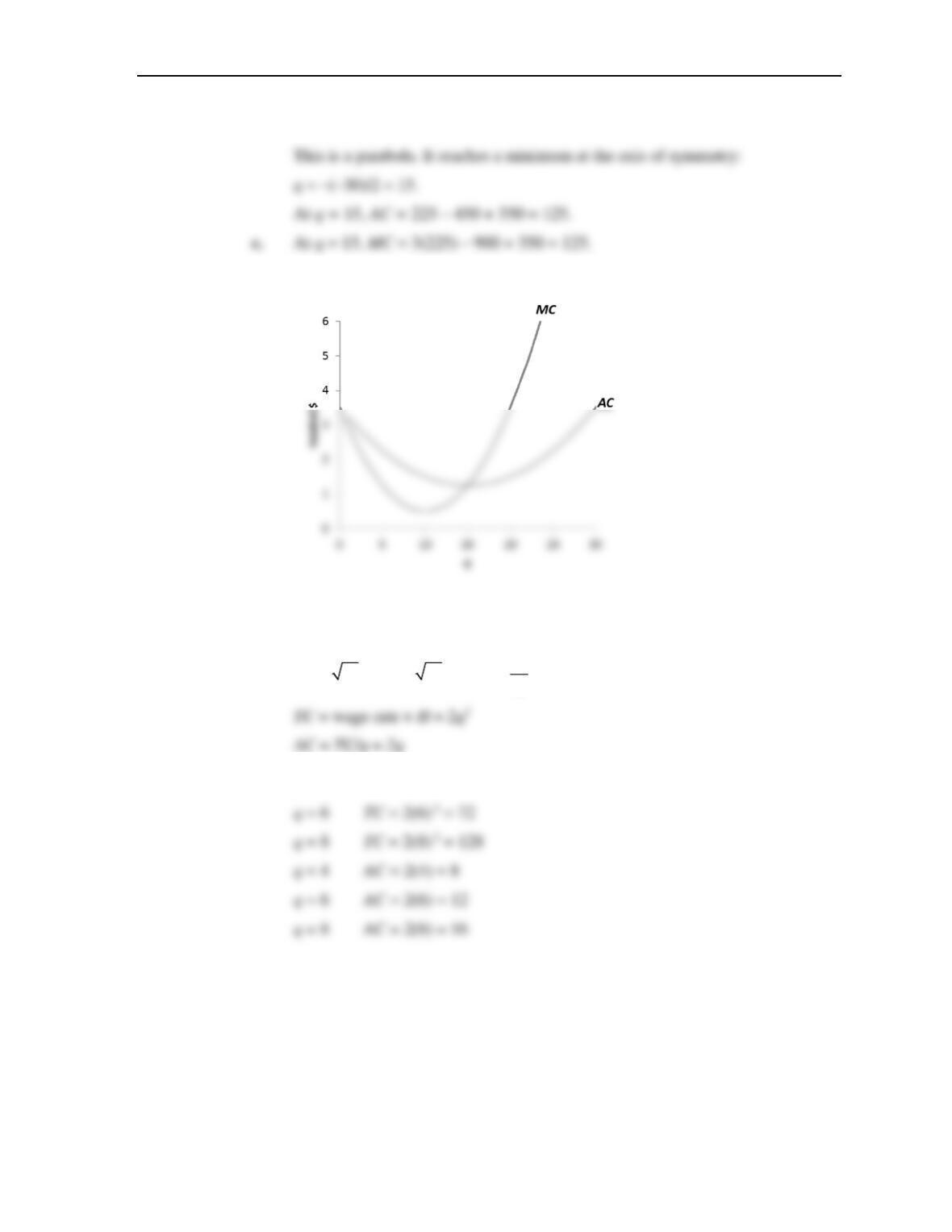
7.3 a. This is a cubic cost curve, resembling Figure 7.3(d).
Chapter 7: Costs
5
b. AC = TC/q = q2 – 30q + 350.
d.
7.4 a. q = 2
H
q/2 =
H
2
4
q
H=
b. q = 4 TC = 2(4)2 = 32
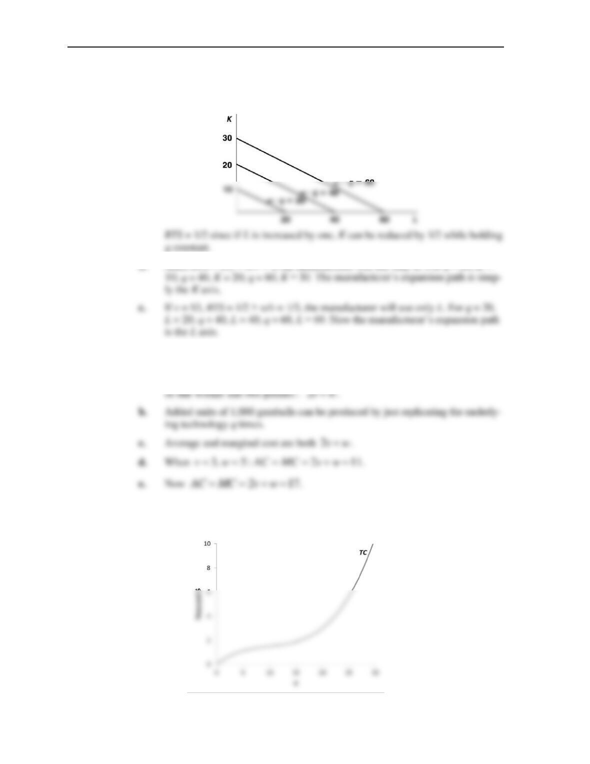
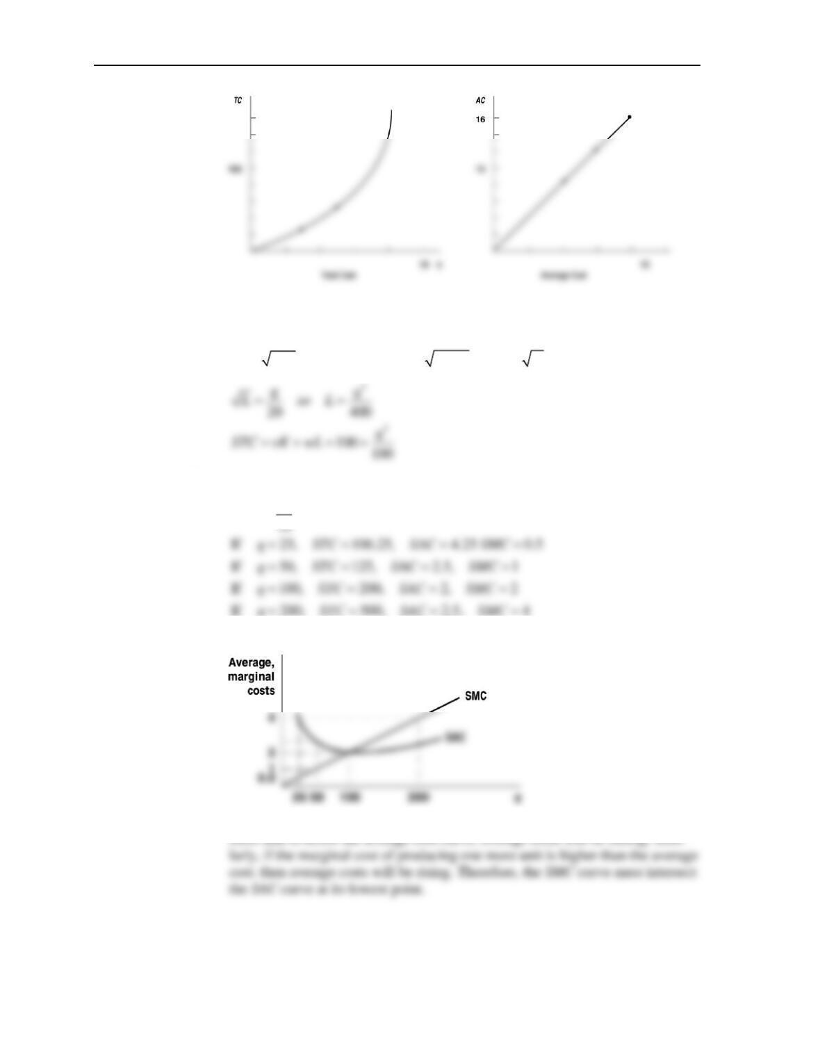
c. The TC and AC curves are shown in the graph. Notice that the convex shape of
TC implies that AC is always increasing.
Chapter 7: Costs
6
7.5 a. q = 2
KL
K = 100, q = 2
100 .L
q = 20
.L
b.
q
SMC
=
c.
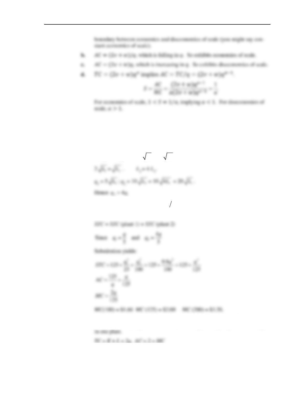
d. The curves intersect at q = 100. As long as the marginal cost of producing one
7.6 a. It is a constant returns to scale production function. The average cost function
𝐴𝐶 = 2𝑣 + 2, which is flat (that is, independent of 𝑞). So this is a case on the
Chapter 7: Costs
7
7.7 To minimize, costs should equate the marginal productivities of labor in each plant. If
labor were more productive in one plant than another, costs could be lowered by
moving workers.
a. MPL1 = MRL2. 5/2
1
L
= 5/
2
L
.
b.
2
11
2
2
(plant 1) 25 25 25
(plant 2) 100 /100
STC wL q
STC q
= + = +
=+
c. In the long run because of constant returns to scale, can change K so it doesn’t
really matter where production occurs. Could split evenly or produce all output
Chapter 7: Costs
8
d. If there were decreasing returns to scale, then should let each firm have equal
7.8 a. With
0.5 0.5
0.5, .a b TC Bqv w= = =
The associated 𝐴𝐶 is flat, so we are right
b. Returns to scale for this production function are measured by 𝑎 + 𝑏, the recip-
rocal of the exponent on q in the 𝑇𝐶 function. If 𝑎 + 𝑏 > 1, implying increas-
If 𝑎 + 𝑏 > 1 (implying we have increasing returns to scale), then 𝑆 > 1 (im-
plying we have economies of scale). If 𝑎 + 𝑏 < 1 (implying we have decreas-
ing returns to scale), then 𝑆 < 1 (implying we have diseconomies of scale). If
𝑎 + 𝑏 = 1 (implying we have constant returns to scale), then 𝑆 = 1 (implying
d. The greater is either one of the exponents the greater will be the exponent for
that input’s unit cost in the total cost function.
e. This function is linear in the logs of the various variables. It is therefore a good
form for linear regression techniques. Note that the coefficient of ln 𝑞 (actually
Chapter 7: Costs
9
7.10 a. Since w/v = 10/10 = 1, the expansion path would be unchanged. All costs
would be twice what they were before: TC = 2q, AC = MC = 2.
b. If w = 20, v = 5, w/v = 4 and the firm will operate on a new expansion path.
Since cost minimization requires
c. Now
20 20 : ( 20) ( 20) ( )( 20).q L K TC vK wL v q w q w v q= = = + = + = +
With v
= w = 10, TC = q. AC = MC = 1. The technical change has totally offset the price
rise in the input prices.