54
CHAPTER 6
TEACHING NOTES
I cover most of Chapter 6, but not all of the material in great detail. I use the example in Table
6.1 to quickly run through the effects of data scaling on the important OLS statistics. (Students
should already have a feel for the effects of data scaling on the coefficients, fitting values, and R–
squared because it is covered in Chapter 2.) At most, I briefly mention beta coefficients; if
students have a need for them, they can read this subsection.
The functional form material is important, and I spend some time on more complicated models
As far as goodness-of-fit, I only introduce the adjusted R-squared, as I think using a slew of
goodness-of-fit measures to choose a model can be confusing to novices (and does not reflect
empirical practice). It is important to discuss how, if we fixate on a high R-squared, we may
wind up with a model that has no interesting ceteris paribus interpretation.
55
SOLUTIONS TO PROBLEMS
6.1 The generality is not necessary. The t statistic on roe2 is only about −.30, which shows that
roe2 is very statistically insignificant. Plus, having the squared term has only a minor effect on
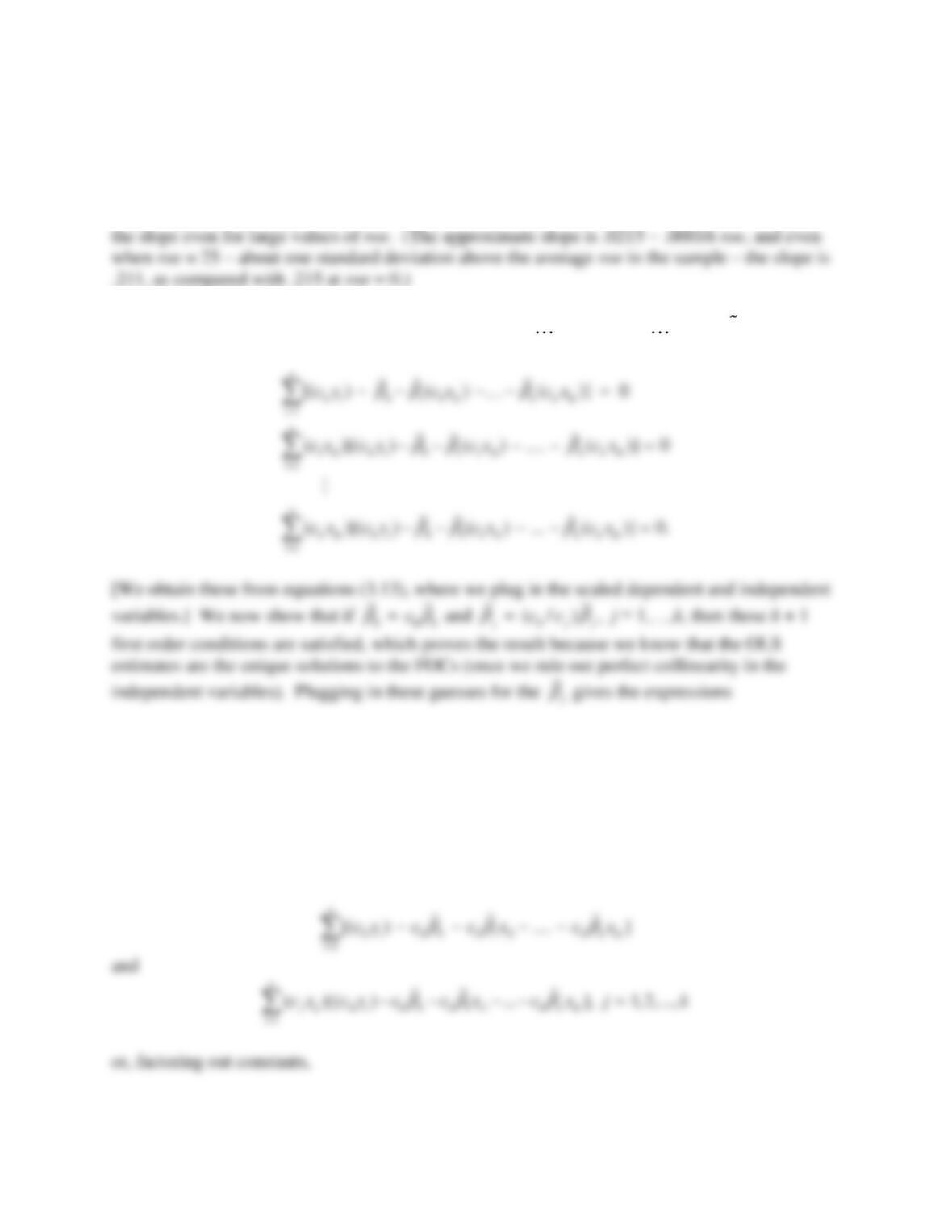
6.2 By definition of the OLS regression of c0yi on c1xi1, , ckxik, i = 2, , n, the
j
solve
0 0 0 0 1 1 1 1 0
1
0 0 0 0 1 1 1 1 0
1
ˆ ˆ ˆ
[( ) ( / ) ( ) … ( / ) ( )]
ˆ ˆ ˆ
( )[( ) ( / ) ( ) … ( / ) ( )],
n
i i k k k ik
i
n
j ij i i k k k ik
i
c y c c c c x c c c x
c x c y c c c c x c c c x
=
=
− − − −
− − − −
for j = 1,2,…,k. Simple cancellation shows we can write these equations as
56
6.3 (i) The turnaround point is given by
1
ˆ
/(2|
2
ˆ
|), or .0003/(.000000014)
21,428.57;
remember, this is sales in millions of dollars.
.036.
(iii) Because sales gets divided by 1,000 to obtain salesbil, the corresponding coefficient gets
(iv) The equation in part (iii) is easier to read because it contains fewer zeros to the right of
6.4 (i) Holding all other factors fixed we have
57
(ii) We use the values pareduc = 32 and pareduc = 24 to interpret the coefficient on educ
6.5 This would make little sense. Performances on math and science exams are measures of
6.6 The extended model has df = 680 – 9 = 671, and we are testing two restrictions. Therefore,
F = [(.232 – .229)/(1 – .232)](671/2)
1.31, which is well below the 10% critical value in the F
6.7 The second equation is clearly preferred, as its adjusted R-squared is notably larger than that
6.8 (i) The answer is not entirely obvious, but one must properly interpret the coefficient on
alcohol in either case. If we include attend, then we are measuring the effect of alcohol
consumption on college GPA, holding attendance fixed. Because attendance is likely to be an
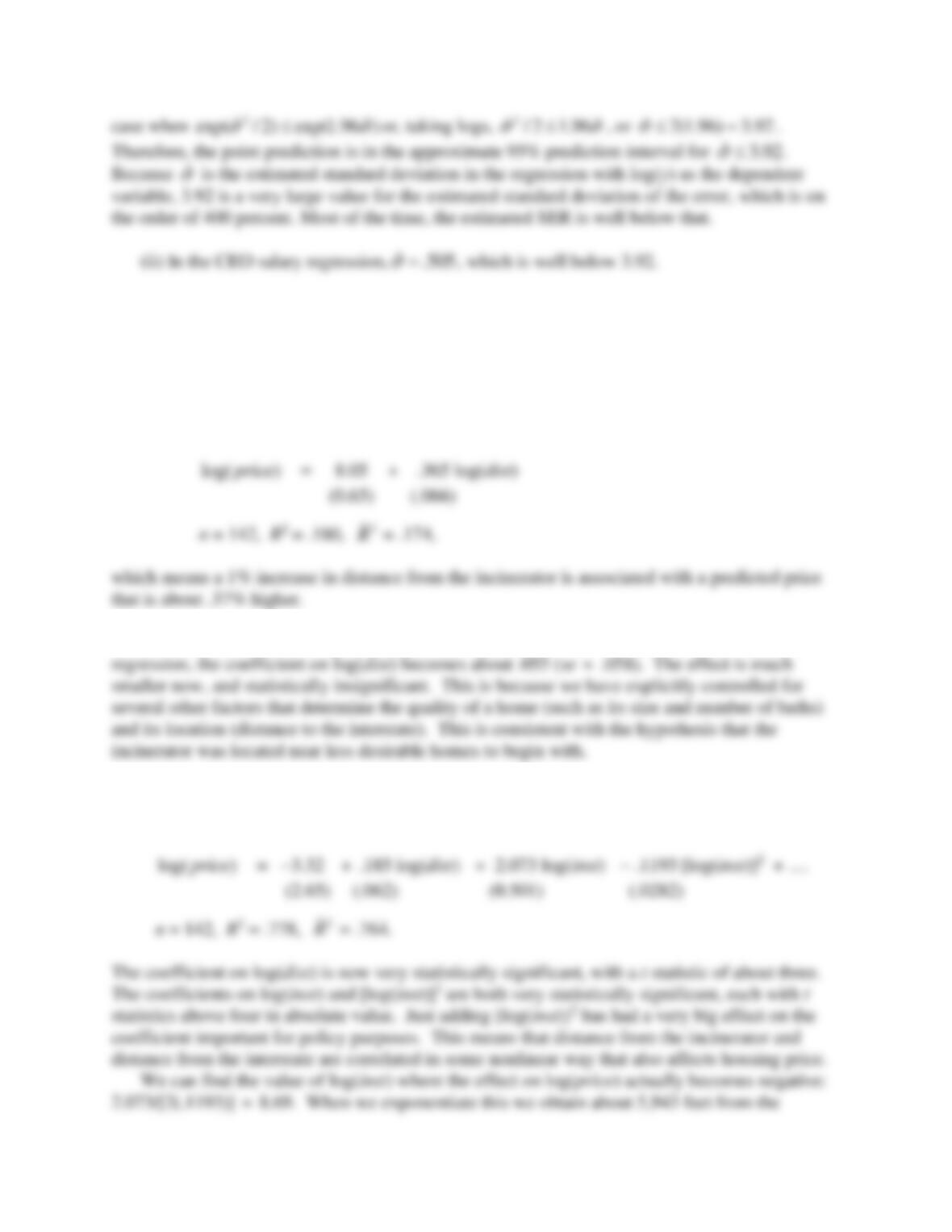
6.9 (i) Because
ˆ
exp( 1.96 ) 1
−
and
2
ˆ
exp( / 2) 1
, the point prediction is always above the
lower bound. The only issue is whether the point prediction is below the upper bound. This is the
58
SOLUTIONS TO COMPUTER EXERCISES
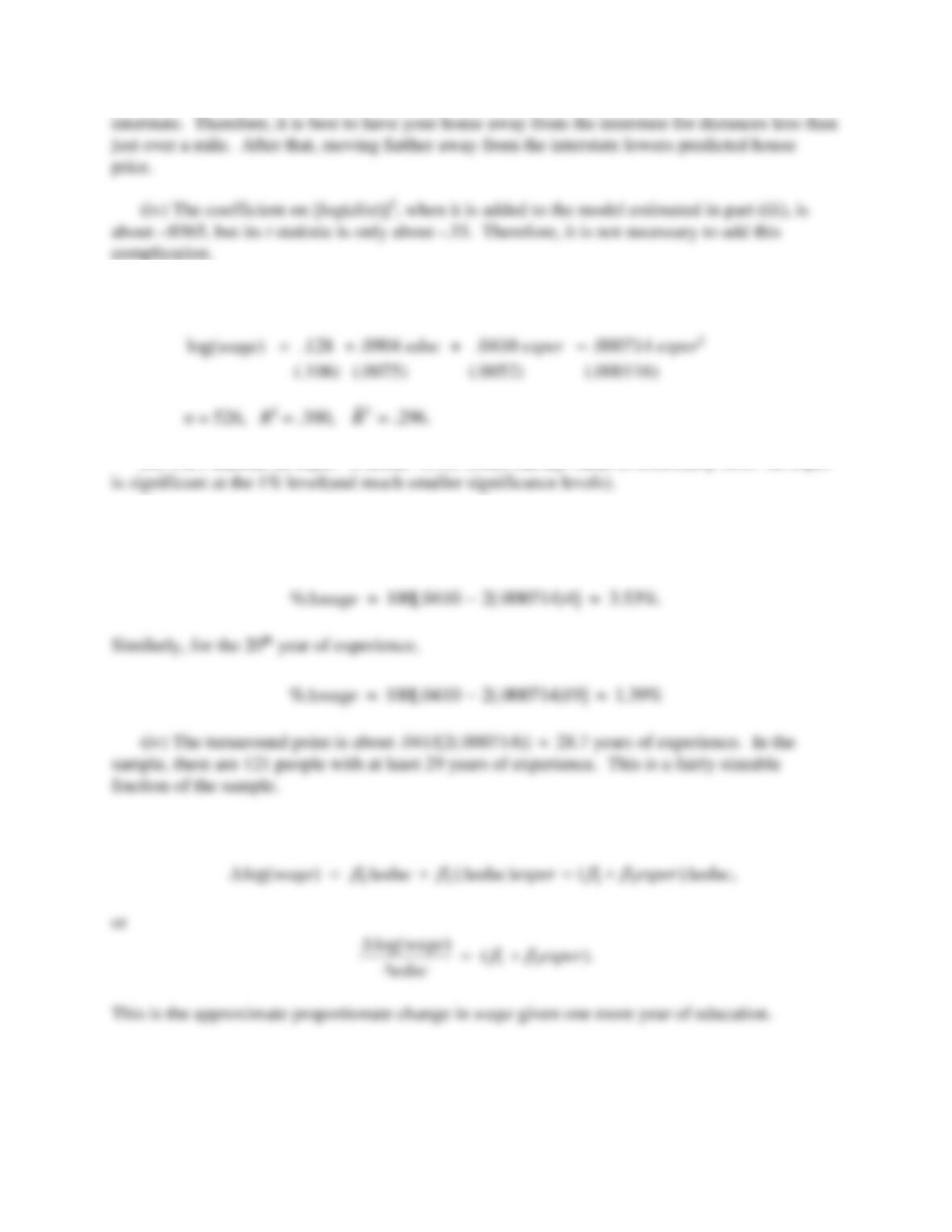
C6.1 (i) The causal (or ceteris paribus) effect of dist on price means that
1
0: all other
relevant factors equal, it is better to have a home farther away from the incinerator. The
estimated equation is
(ii) When the variables log(inst), log(area), log(land), rooms, baths, and age are added to the
(iii) When [log(inst)]2 is added to the regression in part (ii), we obtain (with the results only
partially reported)
59
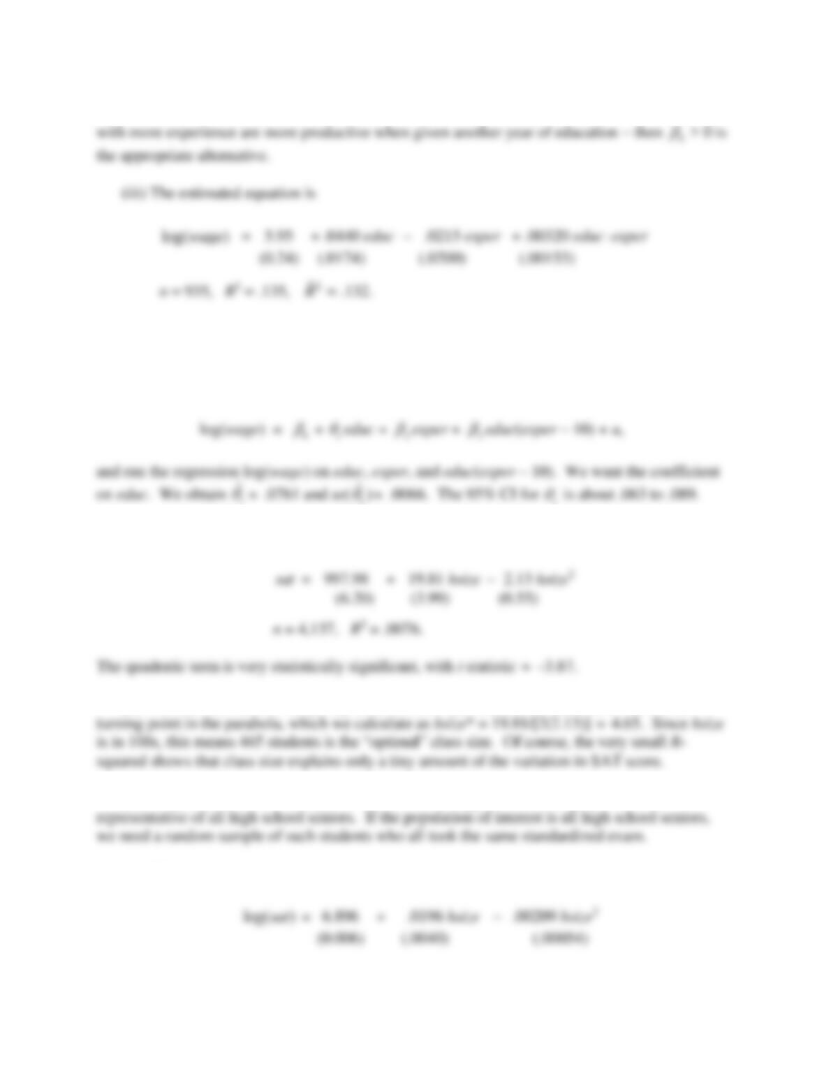
C6.2 (i) The estimated equation is
(ii) The t statistic on exper2 is about –6.16, which has a p-value of essentially zero. So exper
(iii) To estimate the return to the fifth year of experience, we start at exper = 4 and increase
exper by one, so exper = 1:
C6.3 (i) Holding exper (and the elements in u) fixed, we have
60
(ii) H0:
3
= 0. If we think that education and experience interact positively – so that people
The t statistic on the interaction term is about 2.13,which gives a p-value below .02 against H1:
3
> 0. Therefore, we reject H0:
3
= 0 against H1:
3
> 0 at the 2% level.
(iv) We rewrite the equation as
log(wage) =
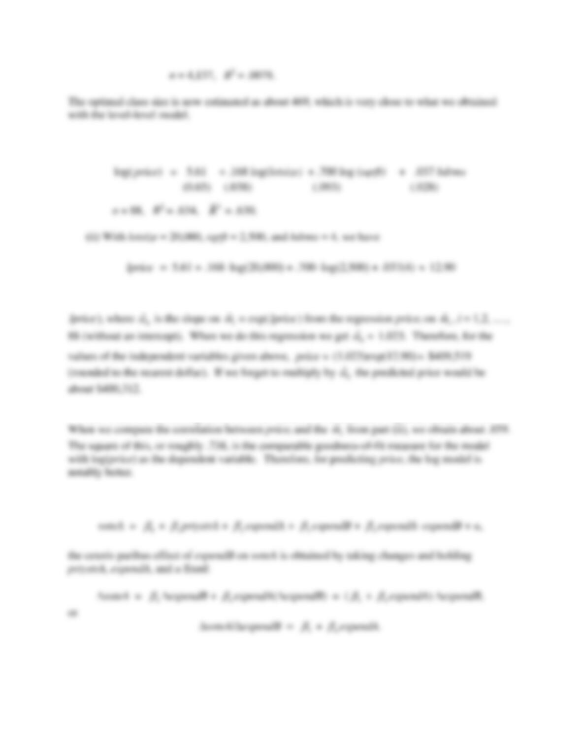
C6.4 (i) The estimated equation is
(ii) We want the value of hsize, say hsize*, where
ˆ
sat
reaches its maximum. This is the
(iii) Only students who actually take the SAT exam appear in the sample, so it is not
(iv) With log(sat) as the dependent variable we get
61
C6.5 (i) The results of estimating the log-log model (but with bdrms in levels) are
where we use lprice to denote log(price). To predict price, we use the equation
ˆ
price
=
0
ˆ
exp(
(iii) When we run the regression with all variables in levels, the R-squared is about .672.
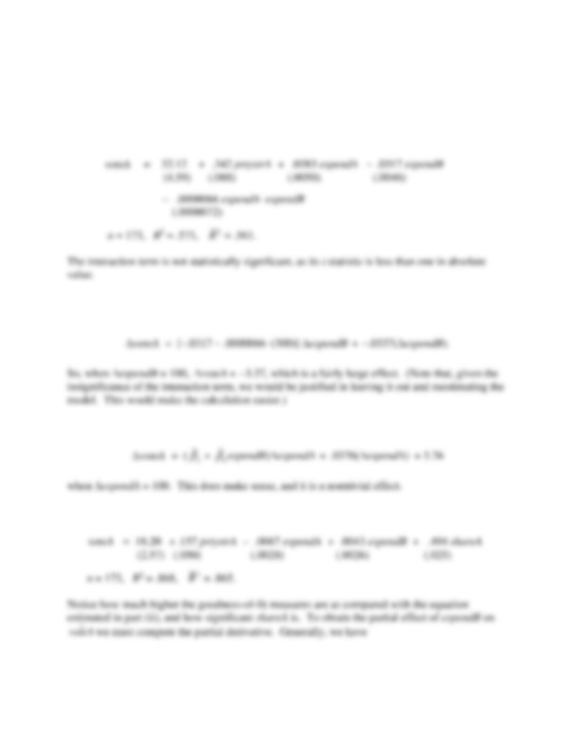
C6.6 (i) For the model
voteA =
62
We think
3
< 0 if a ceteris paribus increase in spending by B lowers the share of the vote
received by A. But the sign of
4
is ambiguous: Is the effect of more spending by B smaller or
larger for higher levels of spending by A?
(ii) The estimated equation is
(iii) The average value of expendA is about 310.61, or $310,610. If we set expendA at 300,
which is close to the average value, we have
(iv) Now we have
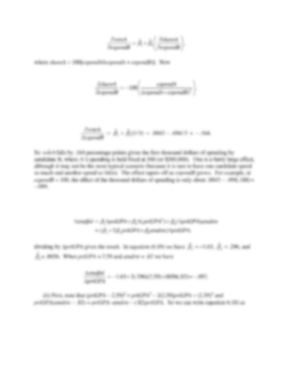
(v) When we replace the interaction term with shareA we obtain
63
Evaluated at expendA = 300 and expendB = 0, the partial derivative is –100(300/3002) = −1/3,
and therefore
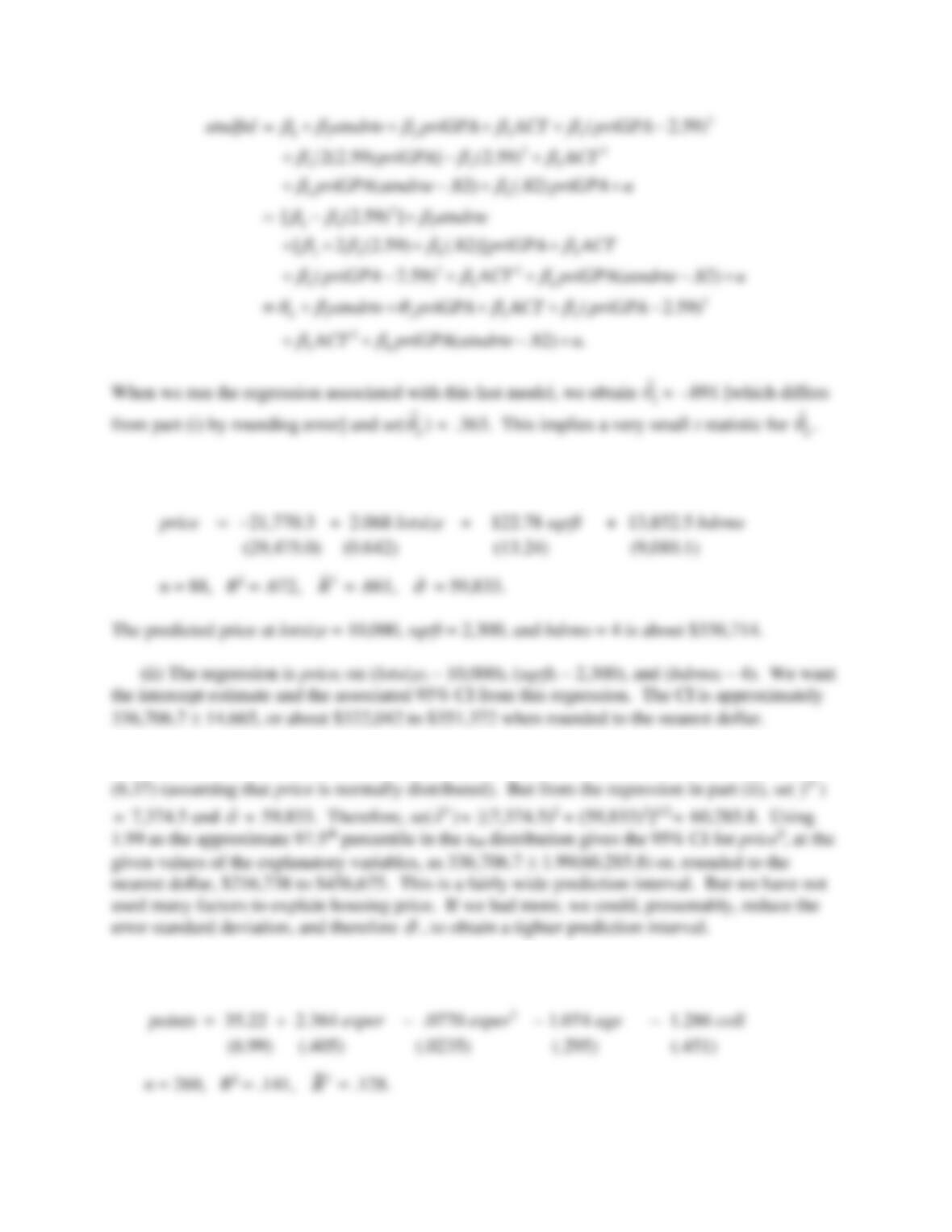
C6.7 (i) If we hold all variables except priGPA fixed and use the usual approximation
(priGPA2)
2(priGPA)priGPA, then we have
64
C6.8 (i) The estimated equation (where price is in dollars) is
(iii) We must use equation (6.36) to obtain the standard error of
0
ˆ
e
and then use equation
C6.9 (i) The estimated equation is
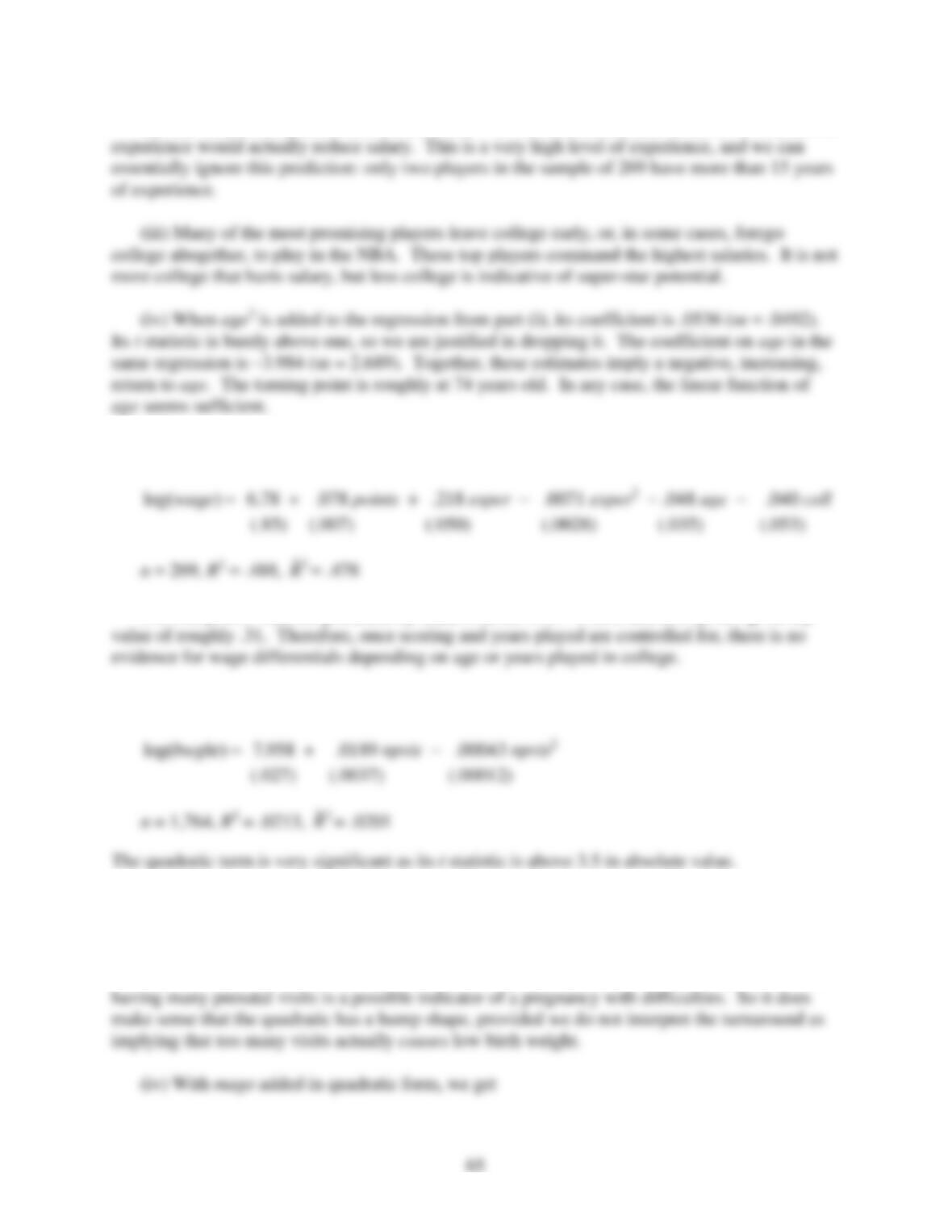
(ii) The turnaround point is 2.364/[2(.0770)] 15.35. So, the increase from 15 to 16 years of
(v) The OLS results are
(vi) The joint F statistic produced by Stata is about 1.19. With 2 and 263 df, this gives a p–
C6.10 (i) The estimated equation is
(ii) The turning point calculation is by now familiar:
*.0189/[2(.00043)] 21.97npvis =
, or
about 22. In the sample, 89 women had 22 or more prenatal visits.
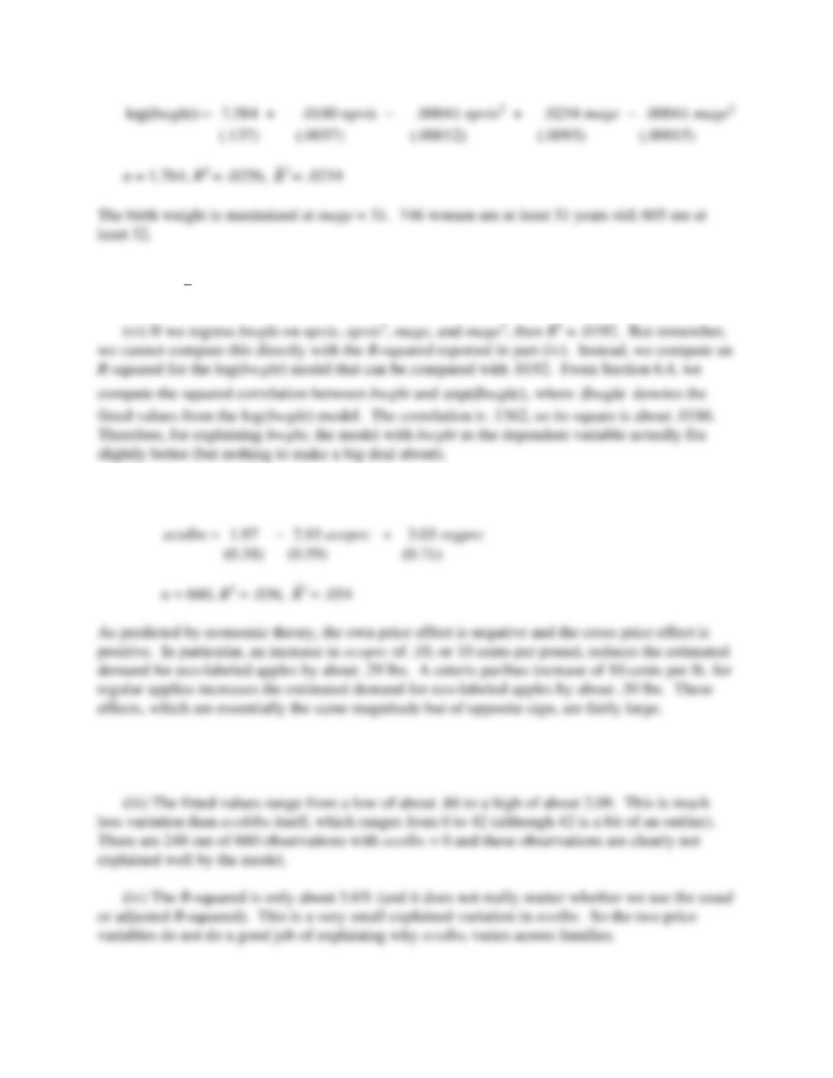
(iii) While prenatal visits are a good thing for helping to prevent low birth weight, a woman’s
66
(v) These variables explain on the order of 2.6% of the variation in log(bwght) (or even less
according to
2
R
), which is not very much.
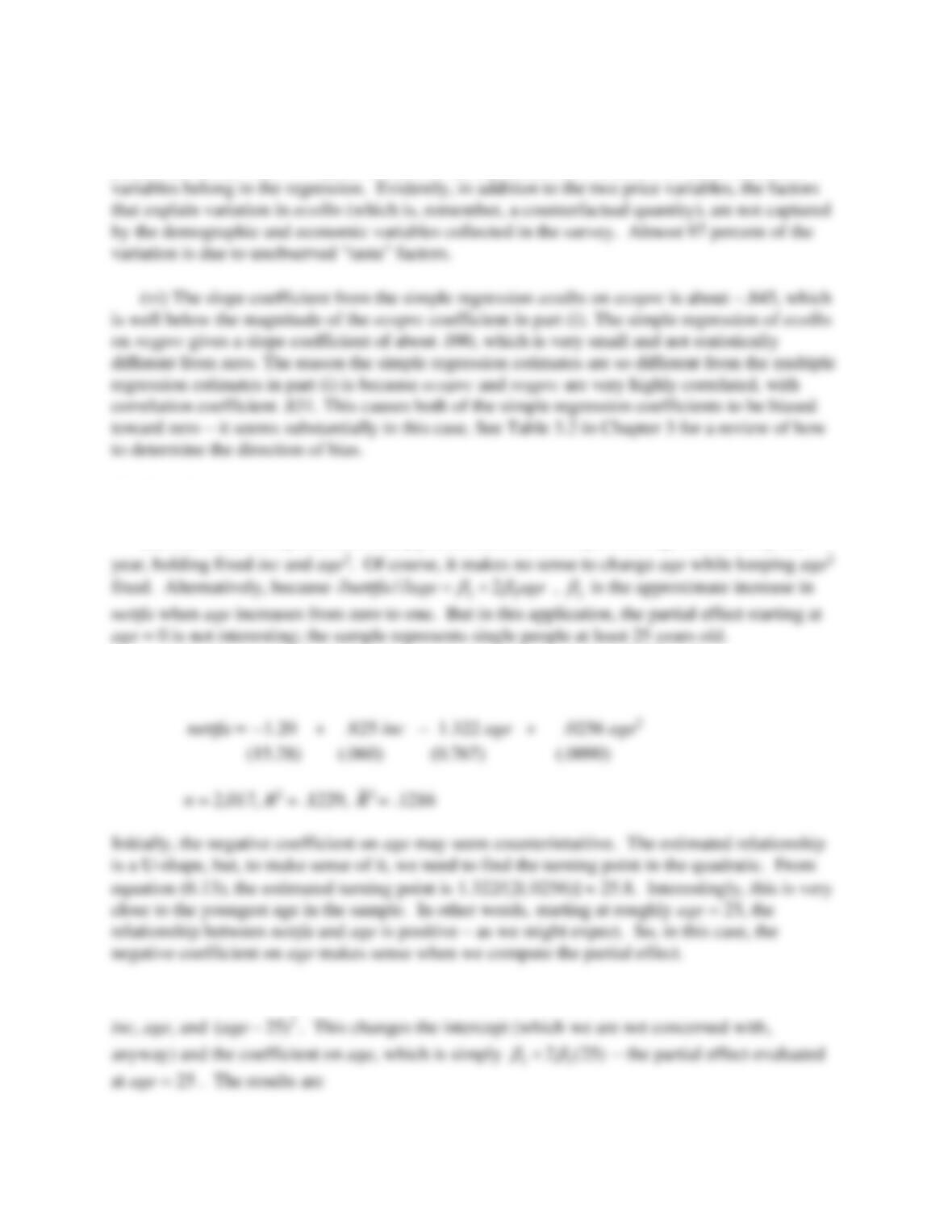
C6.11 (i) The results of the OLS regression are
(ii) Each price variable is individually statistically significant with t statistics greater than
four (in absolute value) in both cases. The p-values are zero to at least three decimal places.
67
(v) When faminc, hhsize, educ, and age are added to the regression, the R-squared only
increases to about .040 (and the adjusted R-squared falls from .034 to .031). The p-value for the
joint F test (with 4 and 653 df) is about .63, which provides no evidence that these additional
C6.12 (i) The youngest age is 25, and there are 99 people of this age in the sample with fsize = 1.
(ii) One literal interpretation is that
2
2
is the increase in nettfa when age increases by one
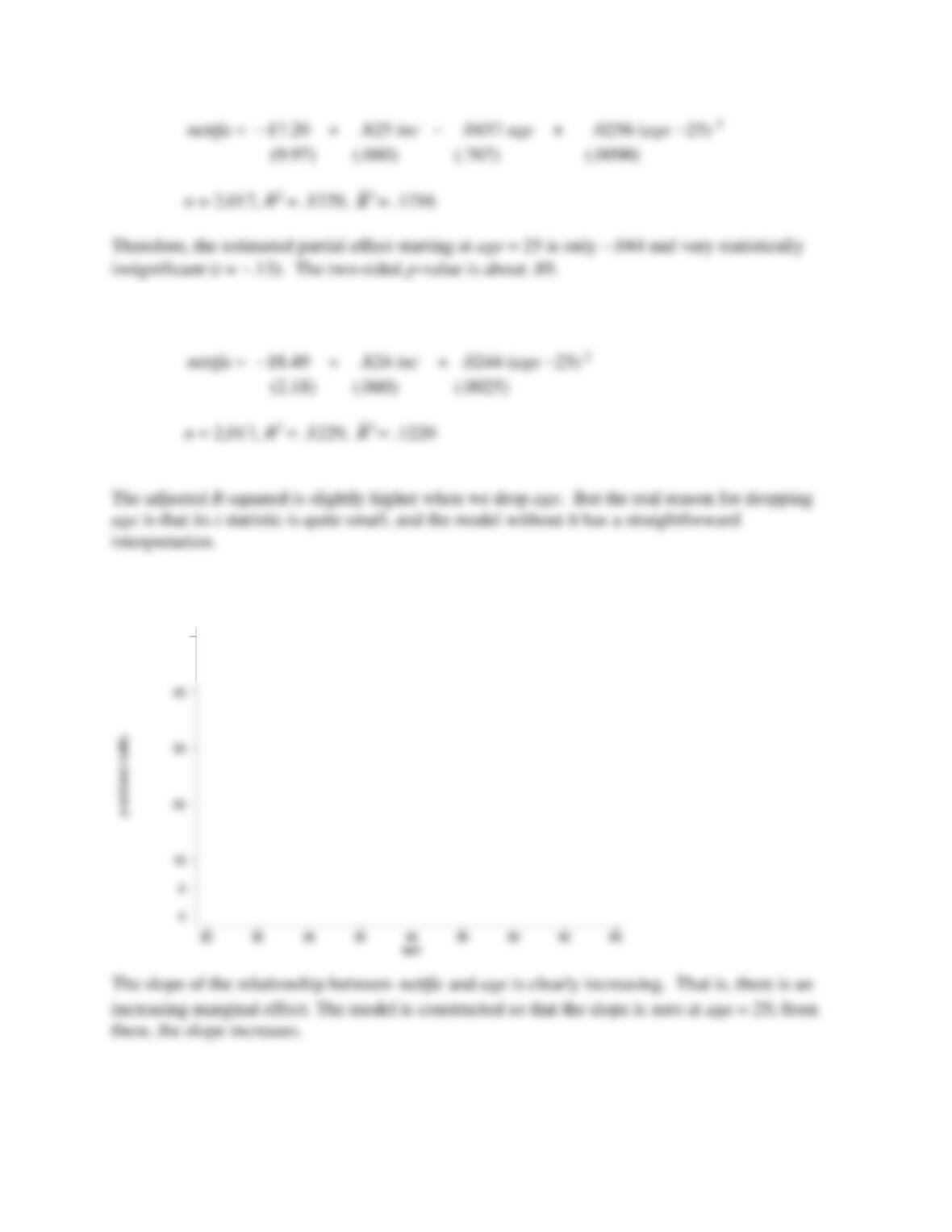
(iii) The OLS estimates are
(iv) I follow the hint, form the new regressor
2
( 25)age −
, and run the regression nettfa on
68
(v) If we drop age from the regression in part (iv) we get
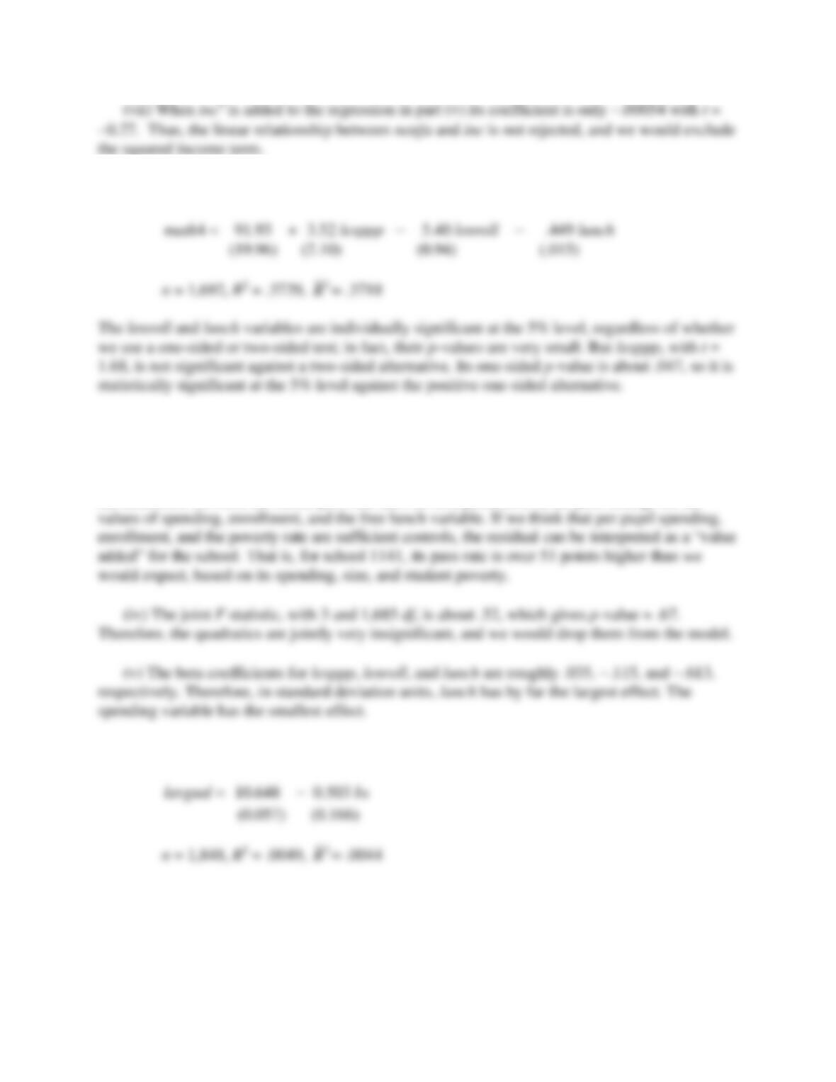
(vi) The graph of the relationship estimated in (v), with inc = 30, is
50
69
C6.13 (i) The estimated equation is
(ii) The range of fitted values is from about 42.41 to 92.67, which is much narrower than the
rage of actual math pass rates in the sample, which is from zero to 100.
(iii) The largest residual is about 51.42, and it belongs to building code 1141. This residual is
the difference between the actual pass rate and our best prediction of the pass rate, given the
C6.14 (i) The simple regression gives
The p-value for testing
0
H : 0
bs
=
against the two-sided alternative is about .002, and so we
easily reject the null. For
0
H : 1
bs
=−
against the one-sided alternative, the p-value is about
.0015, and so we also reject the null.
(ii) The variable lbs = log(bs) ranges from about −2.33 to −.416. Its standard deviation is
(iii) The simple regression of lavgsal on lbs gives an R-squared of .0039, which is less than
(iv) The multiple regression gives
(v) Because the dependent variable is also in logarithmic form, the coefficient on lstaff is
(vi) When lunch2 is added to the equation its coefficient is about .000032 with a t statistic
(vii) The quadratic estimated in part (vi) has a U shape, and so 56.25 is the value of lunch