
Chapter 6
FORECASTING
QUESTIONS AND ANSWERS
Q6.1 Discuss some of the microeconomic and macroeconomic factors a firm must consider in
its own sales and profit forecasting.
Q6.1 ANSWER
The better a company can assess future demand, the better it can plan its resources.
Every corporation is exposed to three types of factors influencing demand: company,
Q6.2 Forecasting the success of new product introductions is notoriously difficult. Describe
some of the macroeconomic and microeconomic factors that a firm might consider in
forecasting sales for a new teeth whitening product.
Q6.2 ANSWER
To forecast market demand for any new product introduction, market size research must
be combined with product-specific information. A useful approach would combine
macroeconomic trend information with data on microeconomic and competitive

140 Chapter 6
Q6.3 Blue Chip Financial Forecasts gives the latest prevailing opinion about the future
direction of the economy. Survey participants include 50 business economists from
Deutsche Banc Alex Brown, Banc of America Securities, Fannie Mae, and other
prominent corporations. Each prediction is published along with the average, or
consensus forecast. Also published are averages of the 10 highest and 10 lowest
forecasts; a median forecast; the number of forecasts raised, lowered, or left unchanged
from a month ago; and a diffusion index that indicates shifts in sentiment that sometimes
occur prior to changes in the consensus forecast. Explain how this approach helps limit
the steamroller or bandwagon problems of the panel consensus method.
Q6.3 ANSWER
Although the panel consensus method often results in forecasts that embody the
collective wisdom of consulted experts, it can be unfavorably affected by the forceful
personality of one or a few key individuals. To mitigate such problems, the forecasting
Q6.4 “Interest rates were expected to increase by 85% of all consumers in the May 2004
survey, more than ever before,” said Richard Curtin, the Director of the University of
Michigan’s Surveys of Consumers. “More consumers in the May 2004 survey cited the
advantage of obtaining a mortgage in advance of any additional increases in interest
rates than any other time in nearly ten years,” said Curtin. Discuss this statement and
explain why consumer surveys are an imperfect guide to consumer expectations.
Q6.4 ANSWER
Survey data can be highly useful in short-term forecasting when carefully used to elicit
consumer perceptions and attitudes. However, survey data are “soft” when they don’t

Forecasting 141
Q6.5 Explain why revenue and profit data reported by shippers such as FedEx Corp. and
United Parcel Service Inc. can provide useful information about trends in the overall
economy.
Q6.5 ANSWER
Revenue and profit data reported by shippers such as FedEx Corp. and United Parcel
Service Inc. are apt to provide useful information about trends in the overall economy
because the pace of goods shipped is a leading indicator of future sales. In a sense,
Q6.6 In prepared remarks before Congress in mid-2007, Federal Reserve Chairman Ben
Bernanke testified: “The principal source of the slowdown in economic growth … has
been the substantial correction in the housing market. [and] The near-term prospects
for the housing market remain uncertain.” What makes forecasting turning points
difficult? What methods do economists use to forecast turning points in the overall
economy?
Q6.6 ANSWER

All economic data have a strong trend element, and turning points are, by definition,
changes in trend. A basic shortcoming of trend projection is that the method is incapable
Q6.7 Would a linear regression model of the advertising/sales relation be appropriate for
forecasting the advertising levels at which threshold or saturation effects become
prevalent? Explain.
Q6.7 ANSWER
Q6.8 Perhaps the most famous early econometric forecasting firm was Wharton Economic
Forecasting Associates (WEFA), founded by Nobel Prize winner Lawrence Klein. A
spin-off of the Wharton School of the University of Pennsylvania, where Klein taught,
WEFA was merged with Data Resources Inc. in 2001 to form Global Insight. Describe
the data requirements that must be met if econometric analysis is to provide a useful
forecasting tool.
Q6.8 ANSWER
If the statistical analysis of economic relations, or econometrics, is to provide a fruitful
tool for forecasting, a number of important conditions must be met. First, a sufficient
number of sample observations must be available for analysis. For small populations

Forecasting 143
Q6.9 Cite some examples of forecasting problems that might be addressed using regression
analysis of complex multiple-equation systems of economic relations.
Q6.9 ANSWER
Econometric analysis of multiple-equation systems of economic relations is a forecasting
technique that is useful for reflecting the effects of important economic changes on
Q6.10 What are the main characteristics of accurate forecasts?
Q6.10 ANSWER
The main characteristics of accurate forecasts are a close correspondence, on average,
SELF-TEST PROBLEMS AND SOLUTIONS
ST6.1 Gross Domestic Product (GDP) is a measure of overall activity in the economy. It is
defined as the value at the final point of sale of all goods and services produced during a
given period by both domestic and foreign-owned enterprises. GDP data for the 1950-
2004 period shown in Figure 6.3 offer the basis to test the abilities of simple constant
change and constant growth models to describe the trend in GDP over time. However,
regression results generated over the entire 1950-2004 period cannot be used to

144 Chapter 6
50-year test period, and a 2000-04 5-year forecast period. Regression models estimated
over the 1950-99 test period can be used to “forecast” actual GDP over the 2000-04
period. In other words, estimation results over the 1950-99 subperiod provide a
forecast model that can be used to evaluate the predictive reliability of the constant
growth model over the 2000-04 forecast period.
A. Use the regression model approach to estimate the simple linear relation between
the natural logarithm of GDP and time (T) over the 1950-99 subperiod, where
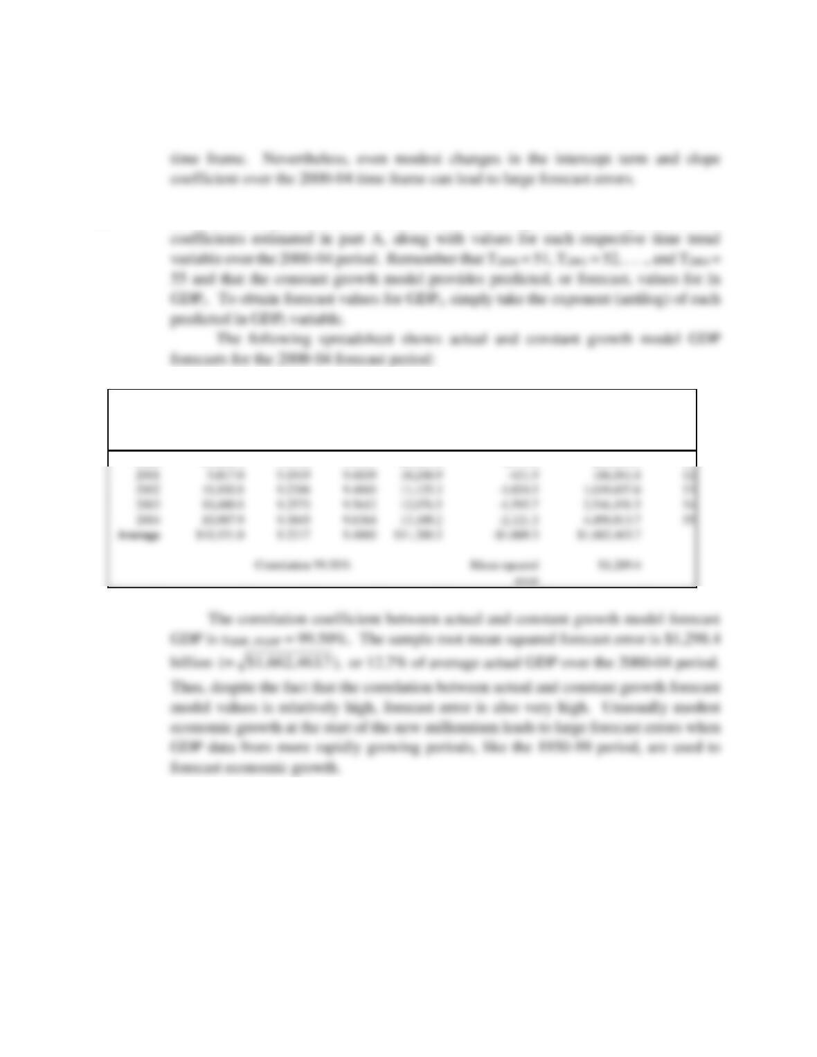
B. Create a spreadsheet that shows constant growth model GDP forecasts over the
2000-04 period alongside actual figures. Then, subtract forecast values from
actual figures to obtain annual estimates of forecast error, and squared forecast
error, for each year over the 2000-04 period.
Finally, compute the correlation coefficient between actual and forecast
values over the 2000-04 period. Also compute the sample average (or root mean
ST6.1 SOLUTION
A. The constant growth model estimated using the simple regression model technique
illustrates the linear relation between the natural logarithm of GDP and time. A constant
Forecasting 145
B. Each constant growth GDP forecast is derived using the constant growth model
Year
GDP
ln GDP
Forecast ln
GDP
Forecast
GDP
Forecast Error
(GDP -Forecast
GDP)
Squared Forecast
Error
(GDP – Forecast
GDP)2
Time
Period
2000
$9,268.4
9.1344
9.3357
$9,441.6
-$173.2
$29,994.1
51
9.2217
9.4860
ST6.2 Multiple Regression. Branded Products, Inc., based in Oakland, California, is a
leading producer and marketer of household laundry detergent and bleach products.
About a year ago, Branded Products rolled out its new Super Detergent in 30 regional
markets following its success in test markets. This isn’t just a “me too” product in a
commodity market. Branded Products’ detergent contains Branded 2 bleach, a
successful laundry product in its own right. At the time of the introduction, management
wondered whether the company could successfully crack this market dominated by
Procter & Gamble and other big players.
146 Chapter 6
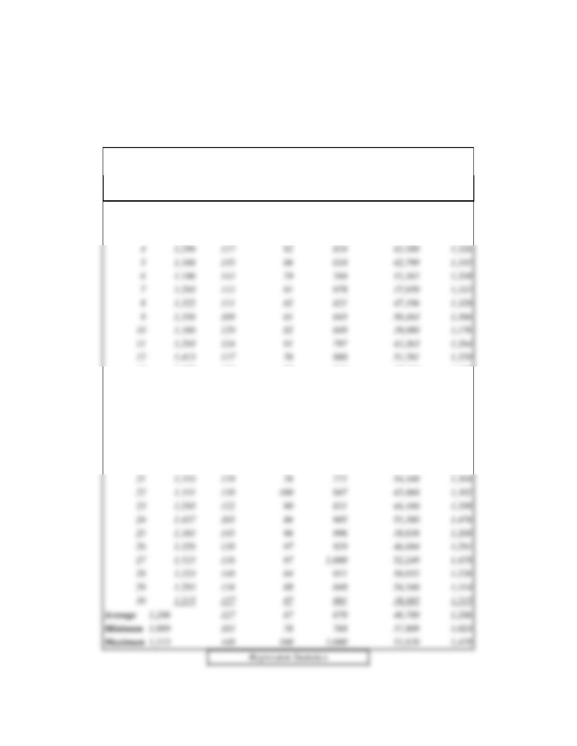
The following spreadsheet shows weekly demand data and regression model
estimation results for Super Detergent in these 30 regional markets:
Branded Products Demand Forecasting Problem
Regional
Market
Demand in
Cases, Q
Price per
Case, P
Competitor
Price, Px
Advertising,
Ad
Household
Income, I
Estimated
Demand, Q
1
1,290
$137
$94
$814
$53,123
1,305
2
1,177
147
81
896
51,749
1,206
3
1,155
149
89
852
49,881
1,204
13
1,299
106
90
914
38,343
1,345
14
1,238
135
88
913
39,473
1,199
15
1,467
117
99
867
51,501
1,433
16
1,089
147
76
785
37,809
1,024
17
1,203
124
83
817
41,471
1,216
18
1,474
103
98
846
46,663
1,449
19
1,235
140
78
768
55,839
1,220
20
1,367
115
83
856
47,438
1,326
21
1,310
119
76
771
54,348
1,304
22
1,331
138
100
947
45,066
1,302
23
1,293
122
90
831
44,166
1,288
24
1,437
105
86
905
55,380
1,476
25
1,165
145
96
996
38,656
1,208
27
1,515
116
97
52,249
1,478
28
1,223
148
84
951
50,855
1,226
29
134
88
848
54,546
1,314
127
87
870
46,788
1,286
103
76
768
37,809
1,024
149
100
55,839
4
117
92
854
43,589
1,326
5
1,166
135
86
810
42,799
1,185
1,186
143
79
768
55,565
1,208
7
1,293
113
91
978
37,959
1,333
8
1,322
111
82
821
47,196
1,328
1,338
109
81
843
50,163
1,366
10
1,160
129
82
39,080
1,176
11
1,293
124
91
797
43,263
1,264
12
1,413
117
76
988
51,291
1,359
Forecasting 147
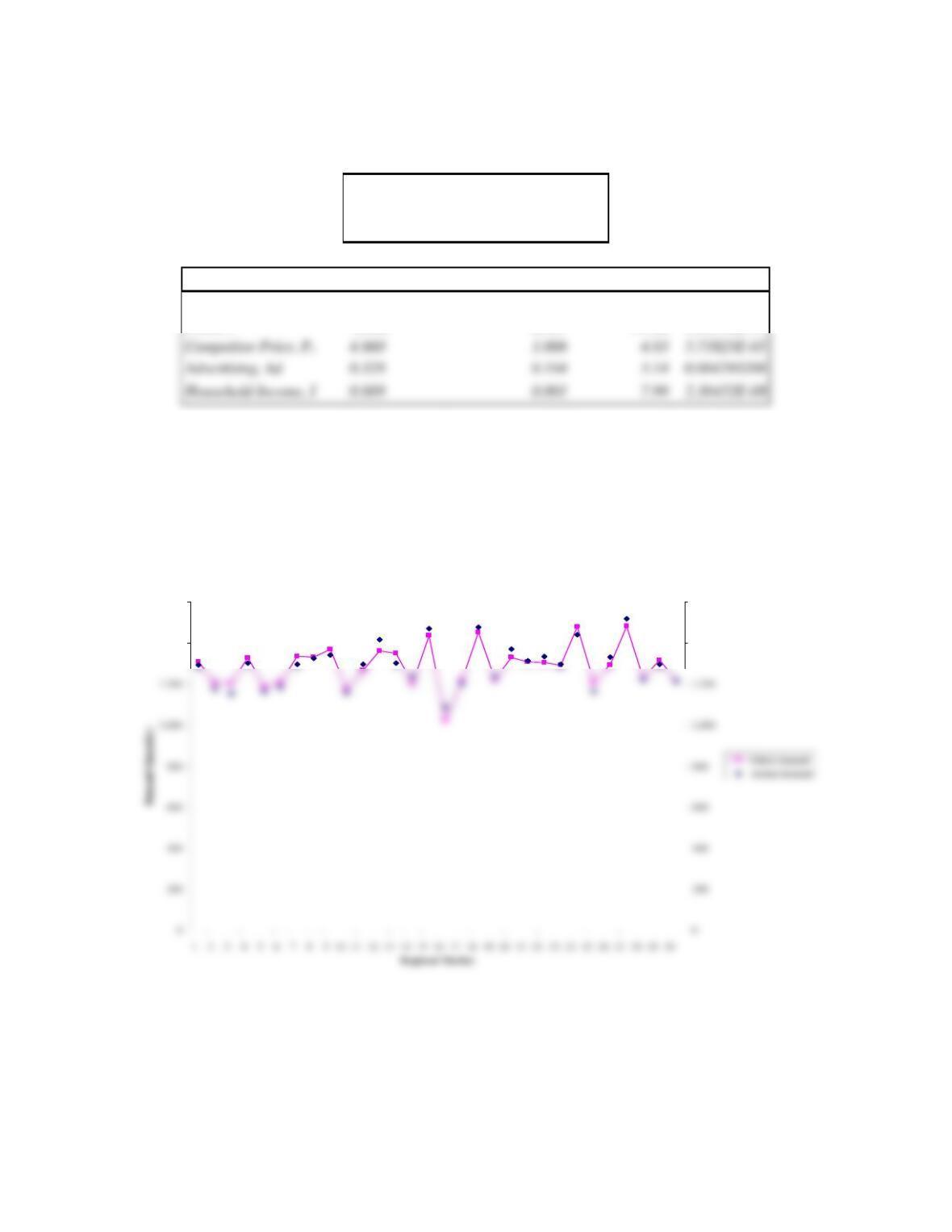
R Square
90.4%
Standard Error
34.97
Observations
30
Coefficients
Standard Error
t Stat
P-value
Intercept
807.938
137.846
5.86
4.09301E-06
Price, P
-5.034
0.457
-11.02
4.34134E-11
A. Interpret the coefficient estimate for each respective independent variable.
B. Characterize the overall explanatory power of this multiple regression model in light
of R2 and the following plot of actual and estimated demand per week.
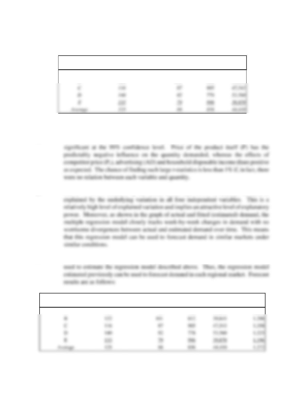
C. Use the regression model estimation results to forecast weekly demand in five new
markets with the following characteristics:
Branded Products Inc. Actual and Fitted Demand
1,400
1,600
1,400
1,600
Competitor Price, Px
4.860
1.006
5.73825E-05
Advertising, Ad
0.328
0.104
148 Chapter 6
Regional Forecast
Market
Price per Case, P
Competitor Price,
Px
Advertising,
Ad
Household
Income, I
A
115
90
790
41,234
B
122
101
812
39,845
ST6.2 SOLUTION
A. Coefficient estimates for the P, Px, Ad and I independent X-variables are statistically
B. The R2 = 90.4% obtained by the model means that 90.4% of demand variation is
C. Notice that each prospective market displays characteristics similar to those of markets
Regional Forecast
Market
Price per
Case, P
Competitor
Price, Px
Advertising,
Ad
Household
Income, I
Forecast
Demand, Q
A
115
90
790
41,234
1,285
140
82
778
53,560
1,223
C
116
87
905
47,543
140
82
778
53,560
Forecasting 149
PROBLEMS AND SOLUTIONS
P6.1 Constant Growth Model. The U.S. Bureau of the Census publishes employment statistics
and demand forecasts for various occupations.
Employment
(1,000)
Occupation
1998
2008
A. Using a spreadsheet or hand-held calculator, calculate the ten-year growth rate
forecast using the constant growth model with annual compounding, and the
constant growth model with continuous compounding for each occupation.
B. Compare your answers and discuss any differences.
P6.1 SOLUTION
A. Using the assumption of annual compounding,
150 Chapter 6
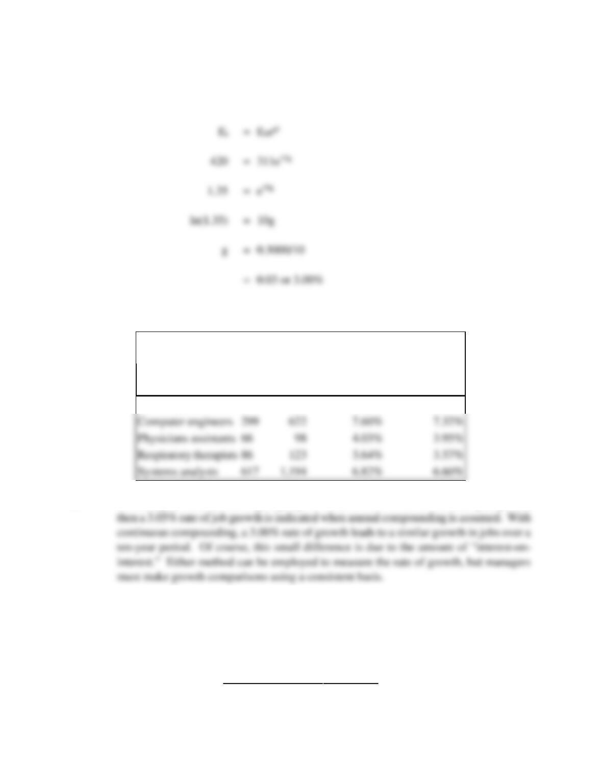
Using the same methods, continuous growth model estimates for various occupations are:
Employment
(1,000)
Continuous Growth Model
Occupation
1998
2008
Annual
Compounding
Continuous
Compounding
Bill collectors
311
420
3.05%
3.00%
B. For example, if the number of jobs jumps to 420,000 from 311,000 over a ten-year period,
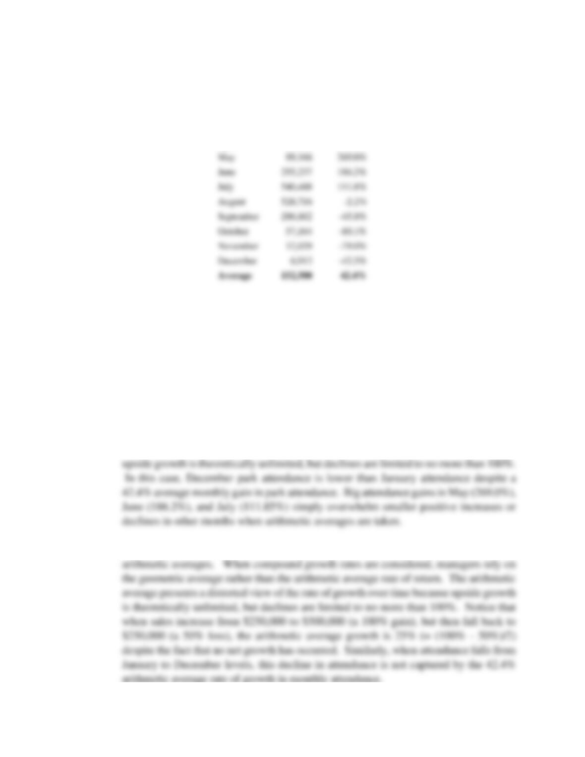
P6.2 Growth Rate Estimation. Almost 2 million persons per year visit wondrous Glacier
National Park. Due to the weather, monthly park attendance figures varied widely during
a recent year:
Month
Visitors
Percent
change
January
7,481
Forecasting 151
February
9,686
29.5%
March
13,316
37.5%
April
24,166
81.5%
A. Notice that park attendance is lower in December than in January, despite a
42.4% average rate of growth in monthly attendance. How is that possible?
B. Suppose the data described in the table measured park attendance over a number
of years rather than during a single year. Explain how the arithmetic average
annual rate of growth gives a misleading picture of the growth in park attendance.
P6.2 SOLUTION
A. The arithmetic average presents a distorted view of the rate of growth over time because
B. This simple example documents the difficulty involved with measuring growth using
June
July
August
September
October
November
12,029
December
152 Chapter 6
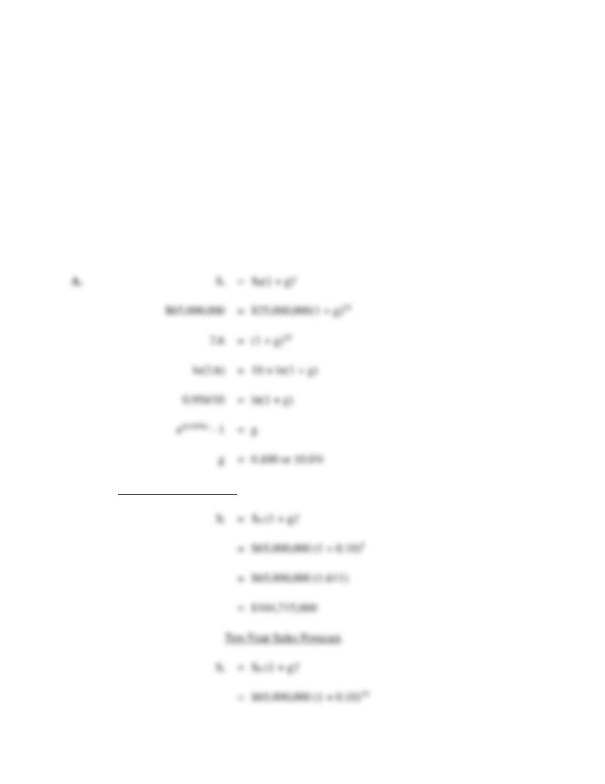
P6.3 Sales Trend Analysis. Environmental Designs, Inc., produces and installs energy-
efficient window systems in commercial buildings. During the past ten years, sales
revenue has increased from $25 million to $65 million.
A. Calculate the company’s growth rate in sales using the constant growth model
with annual compounding.
B. Derive a five-year and a ten-year sales forecast.
P6.3 SOLUTION
B. Five-Year Sales Forecast