Basic Econometrics, Gujarati and Porter
48
CHAPTER 6:
EXTENSIONS OF THE TWO-VARIABLE LINEAR REGRESSION
MODEL
6.1 True. Note that the usual OLS formula to estimate the intercept is
6.2
(
a
) & (
b
) In the first equation an intercept term is included.
(
c
) For each model, a one percentage point increase in the monthly
(
d
) As discussed in the chapter, this model represents the
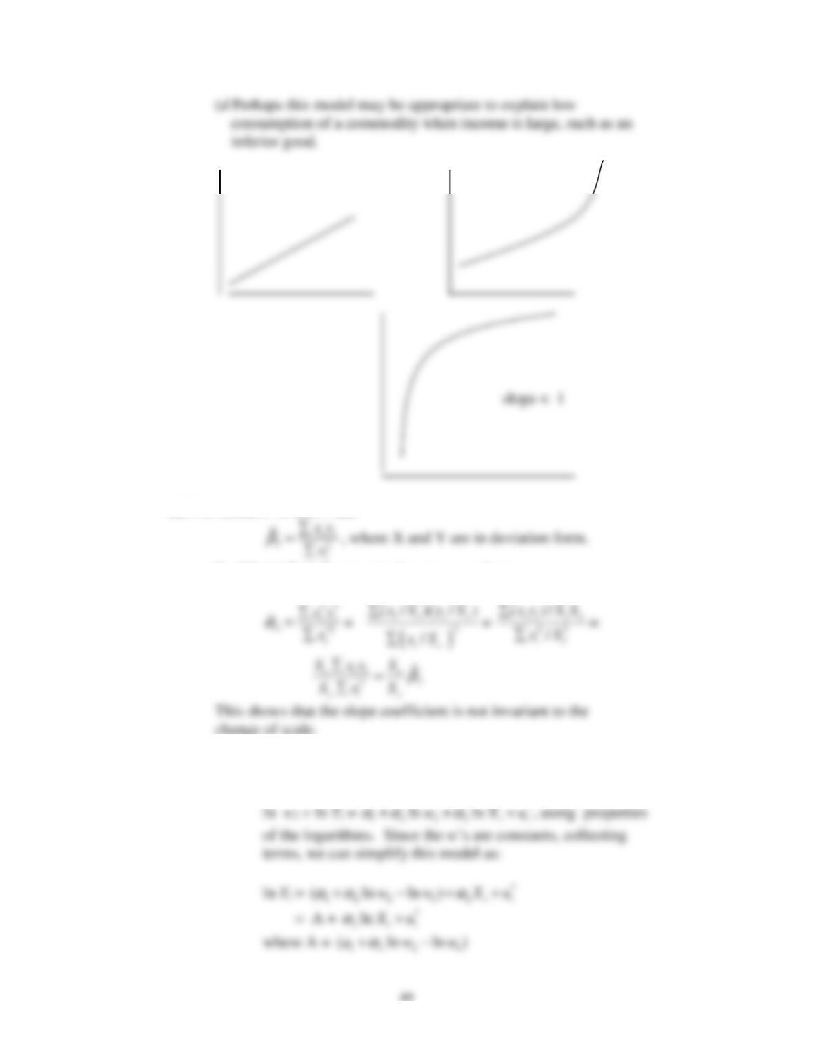
(
f
) Since we have a reasonably large sample, we could use the
(
g
) As per Theil’s remark discussed in the chapter, if the intercept
6.3
(
a
) Since the model is linear in the parameters, it is a linear
Basic Econometrics, Gujarati and Porter
6.4
slope = 1 Slope >1
6.5
For Model I we know that
For Model II, following similar step, we obtain:
6.6
We can write the first model as:
ln (w
1
Y
i
) =
*
1 2 2
ln( )
i i
w X u
α α
+ +
, that is,
50
6.7
Equation (6.6.8) is a growth model, whereas (6.6.10) is a linear
trend model. The former gives the relative change in the
6.8
The null hypothesis is that the true slope coefficient is 0.005.The
alternative hypothesis could be one or two-sided. Suppose we
use the two-sided alternative. The estimated slope value is 0.00705.
Using the
t
test, we obtain:
6.10
As discussed in Sec. 6.7 of the text, for most commodities the
6.11
As it stands, the model is not linear in the parameter. But consider
the following “trick.” First take the ratio of Y to (1-Y) and then take
51
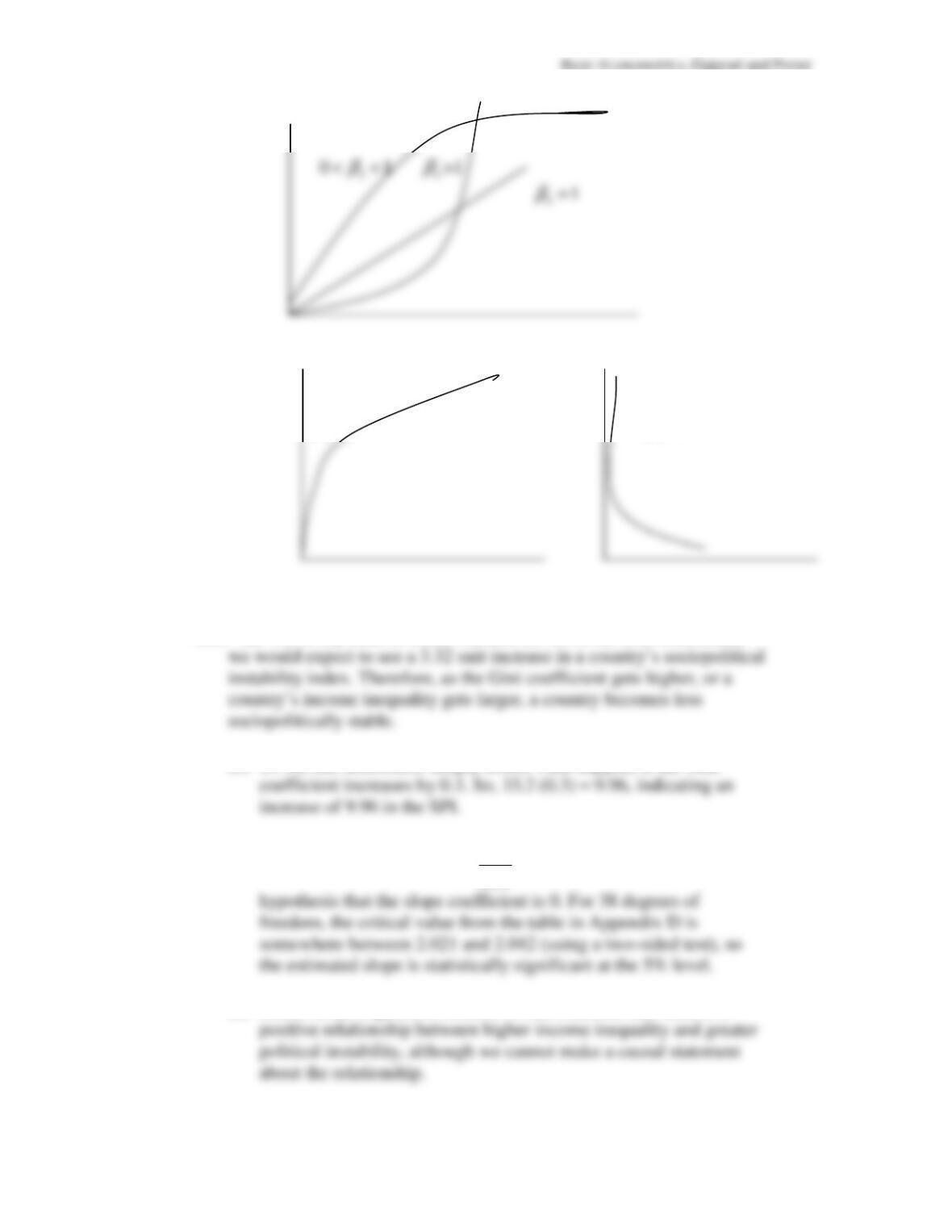
6.12
(
a
)
(b)
2
β
>0
2
β
<0
6.13
(a) For every tenth of a unit increase (0.10) in the Gini coefficient,
(b)
To see this difference, simply assess what happens if the Gini
(c)
Using the standard
t
test,
t
=
33
.
2
1
1
.
8
=
2
.
8136 for testing the null
(d)
Based on the regression results, we can conclude that there is a
Basic Econometrics, Gujarati and Porter
Empirical Exercises
6.14
100
100
Y
=
−
2.0675 + 16.2662
1
X
6.15
(
a
)
(
b
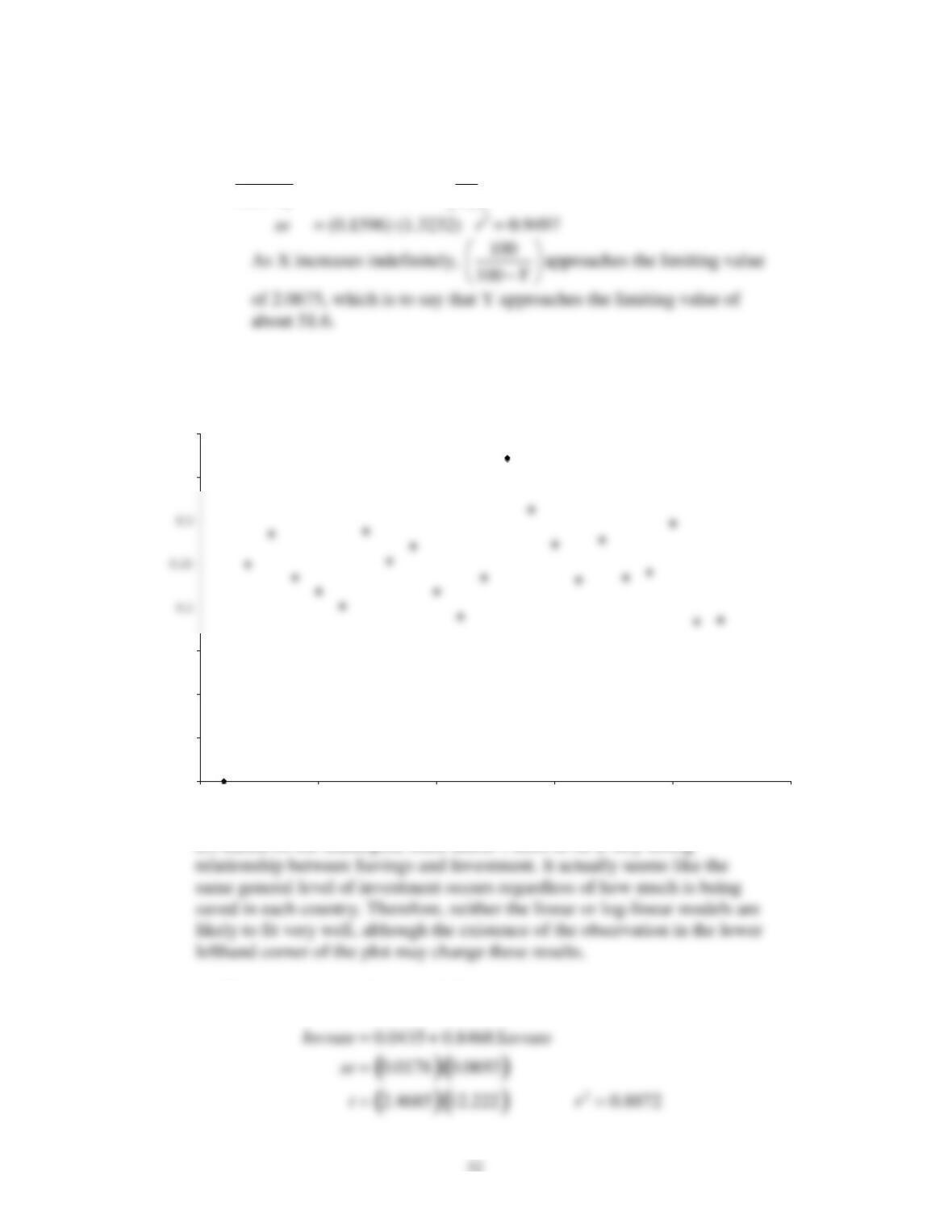
) Based on the scatterplot, there doesn’t seem to be a very strong
(
c
) The regression results are as follows:
Investment vs Savings
0
0.05
0.1
0.15
0.35
0.4
0 5 10 15 20 25
Savings Rate
Basic Econometrics, Gujarati and Porter
53
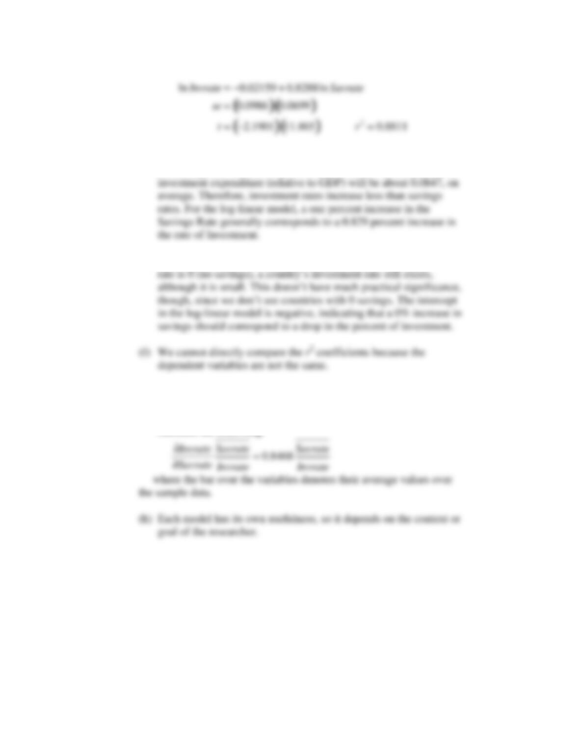
(d)
In the linear model, the slope coefficient can be interpreted as: If
the savings rate increases by 0.1 (relative to GDP), the increase in
(e)
The intercept in the linear model suggests that, when the savings
(g)
For the linear model, the elasticity is not apparent. The log-linear
model, however, already contains the results relative to the
elasticities of the variables. To create the elasticity, we need to
calculate the following:
54
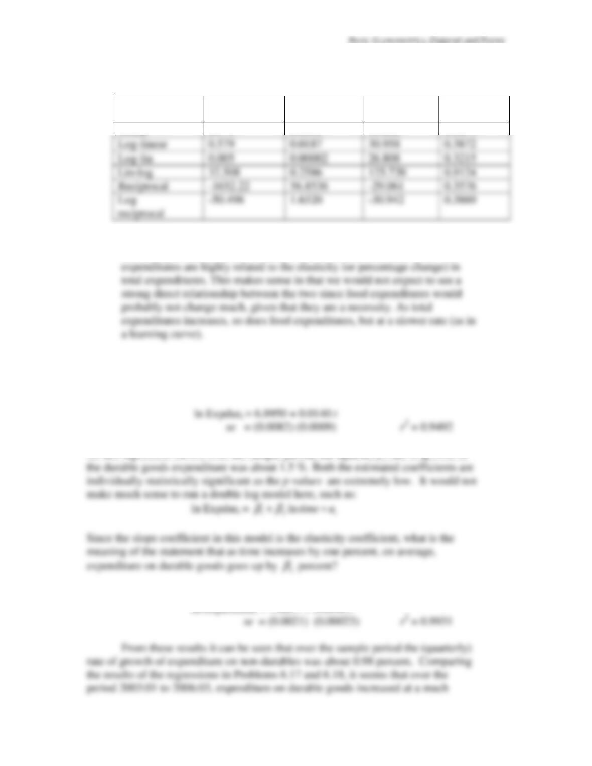
6.16
(
a
)
Model Slope
estimate
se t r
2
Linear 0.173 0.0058 29.666 0.3671
(
b
) We cannot compare the
r
2
values directly, but it does seem that
the lin-log model has the best results. This would indicate that food
To obtain the growth rate of expenditure on durable goods, we can fit the log-
lin model, whose results are as follows:
As this regression shows, over the sample period, the (quarterly) rate of growth in
6.18
The corresponding results for the non-durable goods sector are:
ln Expnondur
= 7.6257 + 0.0098
t
55
6.19
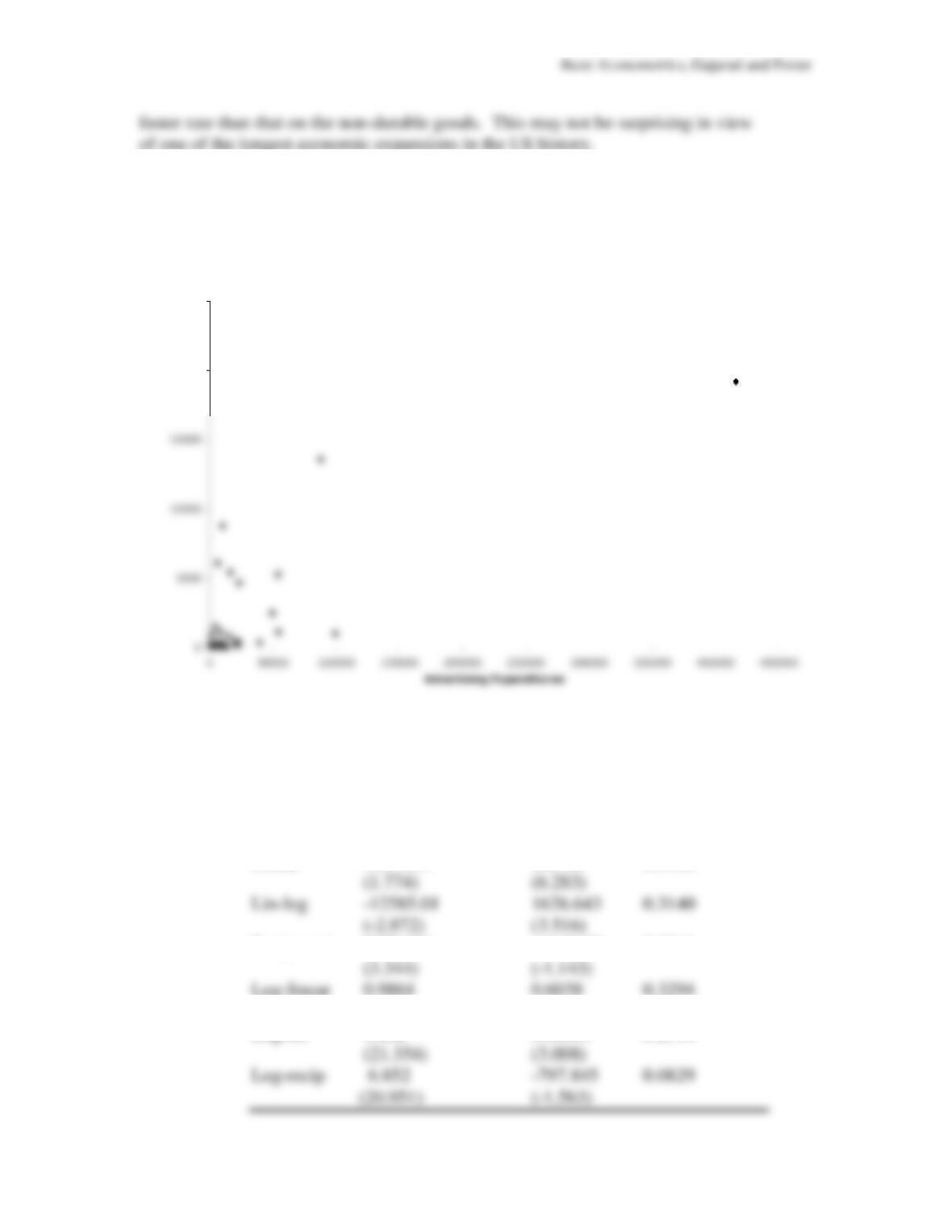
(a) The scattergram of total consumer expenditure and advertising
expenditure is as follows:
(b) Although the relationship between the two variables seems to be
positive, it is not clear which particular curve will fit the data. In the following
table we give regression results based on a few models.
Model Intercept Slope
r
2
_______________________________________________________
Linear 1057.361 0.0446 0.5938
Reciprocal 3077.256 -1642108 0.0461
(0.628) (3.642)
Log-lin 6.262 0.00001 0.2510
Consumer Expenditures vs Advertising Expenditures
20000
25000
Basic Econometrics, Gujarati and Porter
56
Note:
Figures in the parentheses are the estimated
t values.
(c) Assessing the ratio of the variables, it seems there are a few unusually high
6.20
(a)
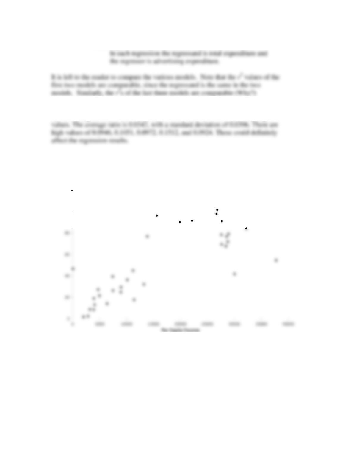
Cellphone Demand vs Per Capita Income
100
120
Basic Econometrics, Gujarati and Porter
57
(b)
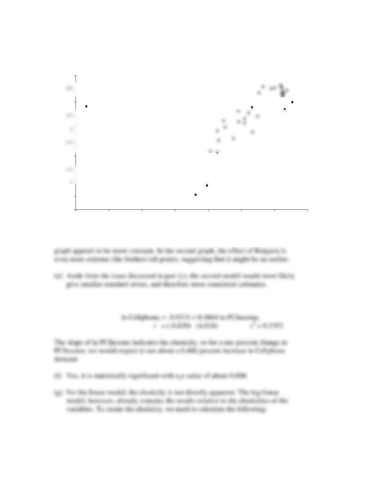
(c) The first graph seems to exhibit non-constant variance, whereas the second
(e)
Double-log regression results are:
Log Cellphone Demand vs Log Income
0
0.5
2
4
5
4 5 6 7 8 9 10 11
Log Per Capita Income
Basic Econometrics, Gujarati and Porter
58
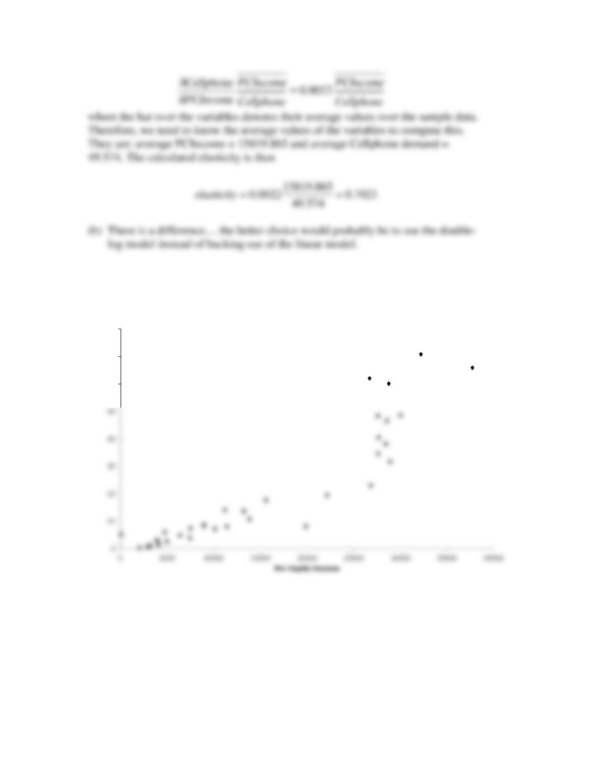
6.21 (a)
PC Demand vs Per Capita Income
60
70
80
Basic Econometrics, Gujarati and Porter
59
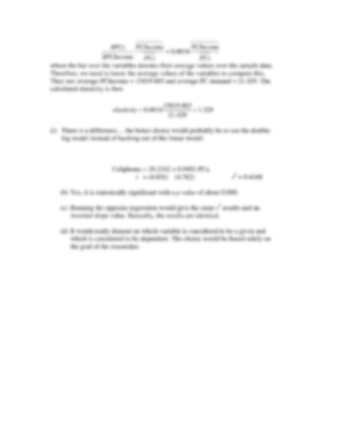
(b)
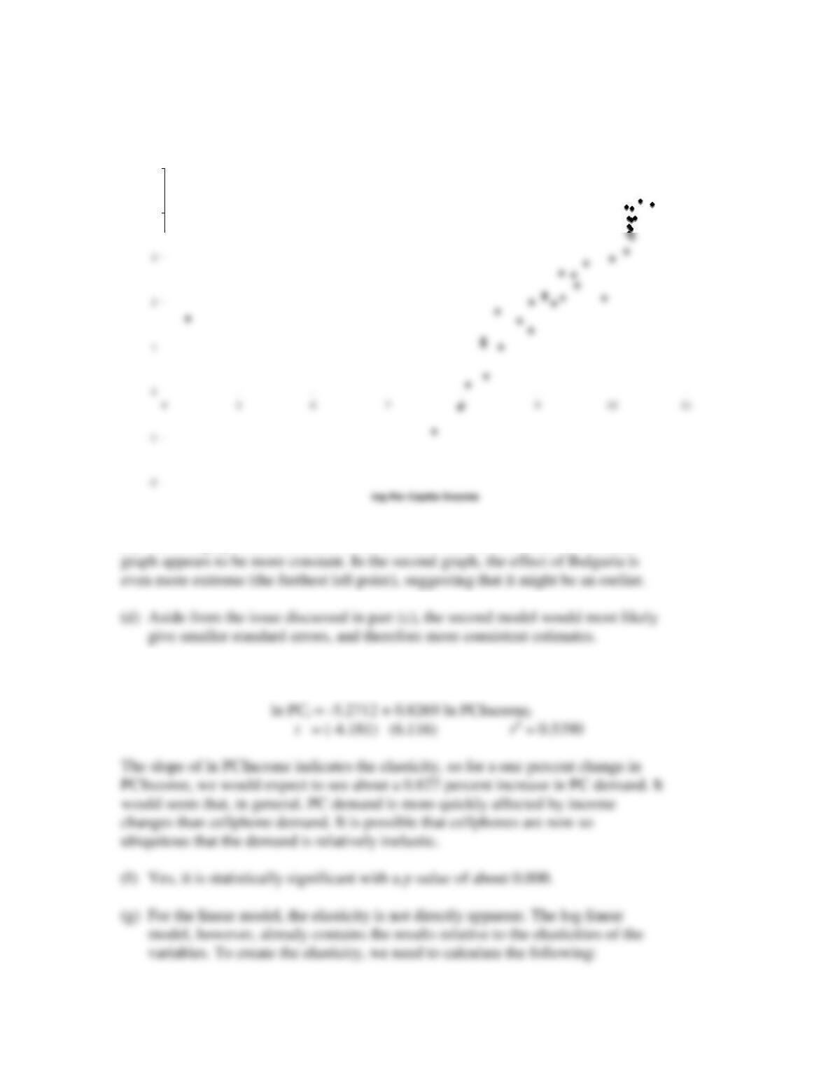
(c) The first graph seems to exhibit non-constant variance, whereas the second
(e) Double-log regression results are:
Log PC Demand vs Log Income
4
5
Basic Econometrics, Gujarati and Porter
60
6.22 (a) Linear regression results are: