Chapter 6
Functional Form and Structural Change
◼ Exercises
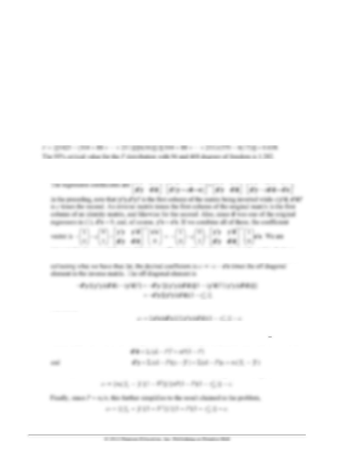
1. The F statistic could be computed as
2. a. Using the hint, we seek the c*, which is the slope on d in the regression of q = y − c d − e on y and d.
()
11
cc
−−
−
y y y d y y d e y y y d y y y d y e
− − −
interested in the second (lower) of the two coefficients. The matrix product at the end is ee times
the first column of the inverse matrix, and we wish to find its second (bottom) element. Therefore,
Therefore,
yd
(The two negative signs cancel.) This can be further reduced. Since all variables are in deviation
form, ee/yy is (1 − R2) in the full regression. By multiplying it out, you can show that
d
= P so that
where n1 is the number of observations which have di = 1. Combining terms once again, we have
Chapter 6 Functional Form and Structural Change 39
b. The problem this creates for the theory is that in the present setting, if, indeed, c is negative,
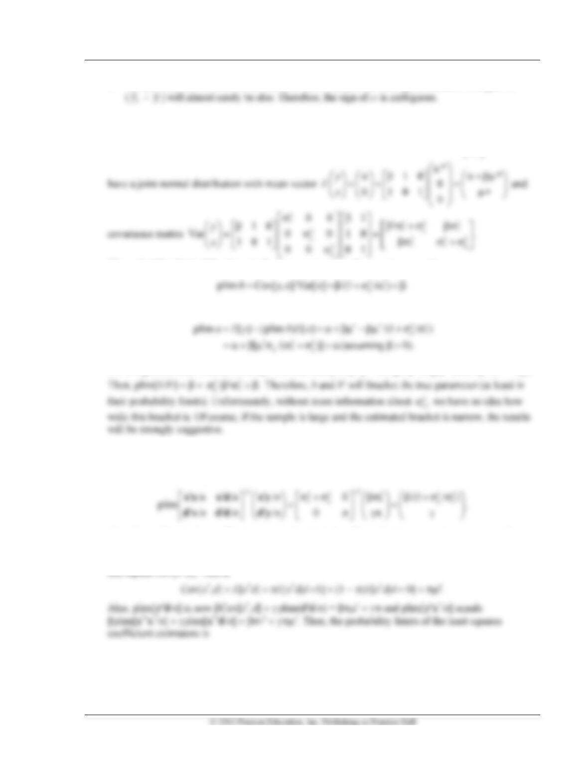
3. We first find the joint distribution of the observed variables
= +
*
0
x
y
xu
so [y, x]
The probability limit of the slope in the linear regression of y on x is, as usual,
The probability limit of the intercept is
If x is regressed on y instead, the slope will estimate plim[b] = Cov[y,x]/Var[y] =
2
*
/(2
2
*
+
2
).
4. In the regression of y on x and d, if d and x are independent, we can invoke the familiar result for
least squares regression. The results are the same as those obtained by two simple regressions.
It is instructive to verify this:
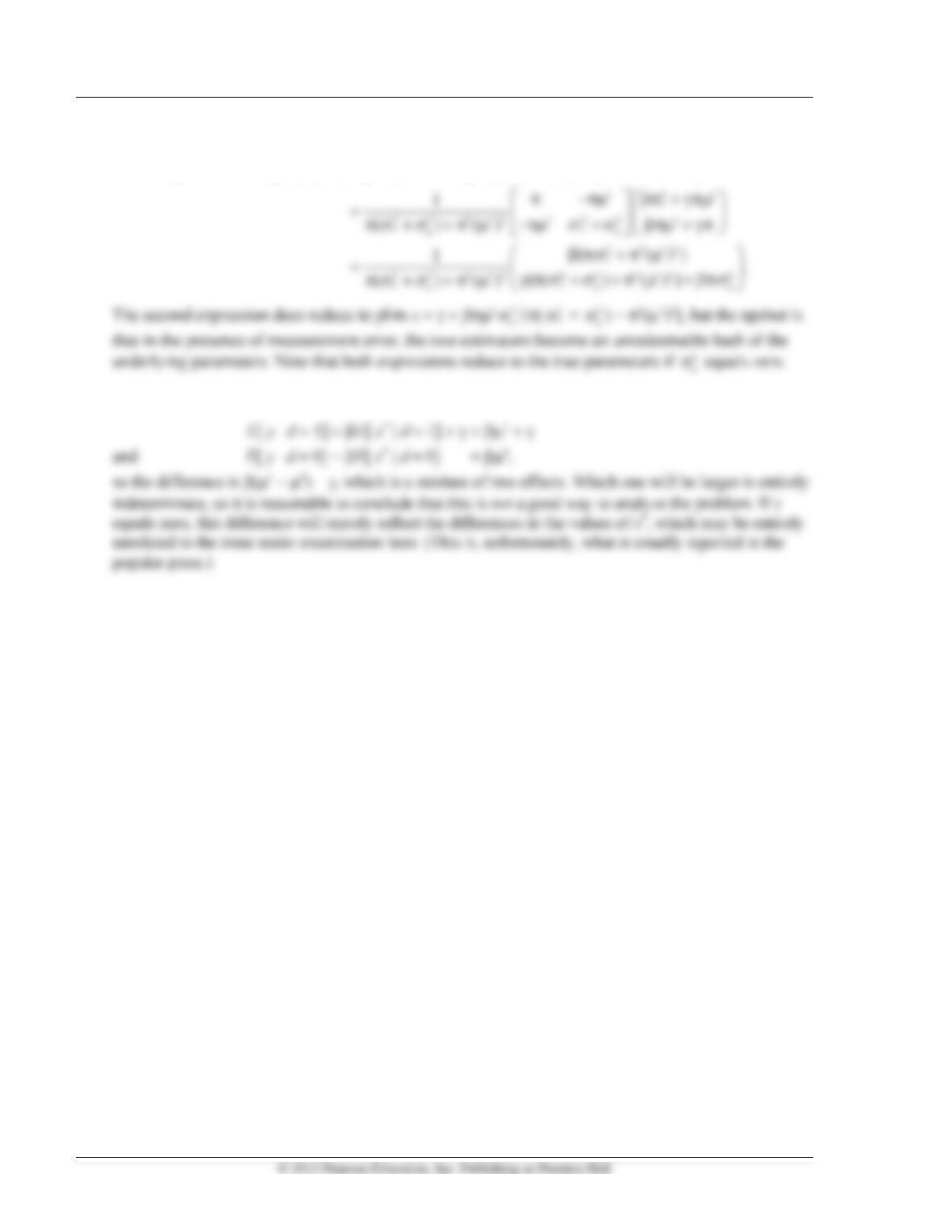
Therefore, although the coefficient on x is distorted, the effect of interest, namely, , is correctly
measured. Now consider what happens if x* and d are not independent. With the second assumption,
we must replace the off diagonal zero above with plim(xd/n). Since u and d are still uncorrelated,
this equals Cov[x*,d]. This is
40 Greene • Econometric Analysis, Seventh Edition
( )
1
122 2
*
/ / / //
plim / / /
uu
n
n
−
−
+ +
+
==
+
x x x d x y
d x d d d y
nn
nn
Finally, the two means are estimators of
Chapter 6 Functional Form and Structural Change 41
Applications
?=======================================================================
? Application 6.1
?=======================================================================
a. Wage equation
Namelist ; X = one,educ,ability,pexp,med,fed,bh,sibs$
Regress ; Lhs = lwage ; Rhs = x $
+—————————————————-+
| Ordinary least squares regression |
| LHS=LWAGE Mean = 2.296821 |
+—————————————————-+
+——–+————–+—————-+——–+——–+———-+
|Variable| Coefficient | Standard Error |b/St.Er.|P[|Z|>z]| Mean of X|
+——–+————–+—————-+——–+——–+———-+
Constant| .96950956 .03370543 28.764 .0000
+————————————+
| Listed Calculator Results |
+————————————+
42 Greene • Econometric Analysis, Seventh Edition
?=======================================================================
? b.
?=======================================================================
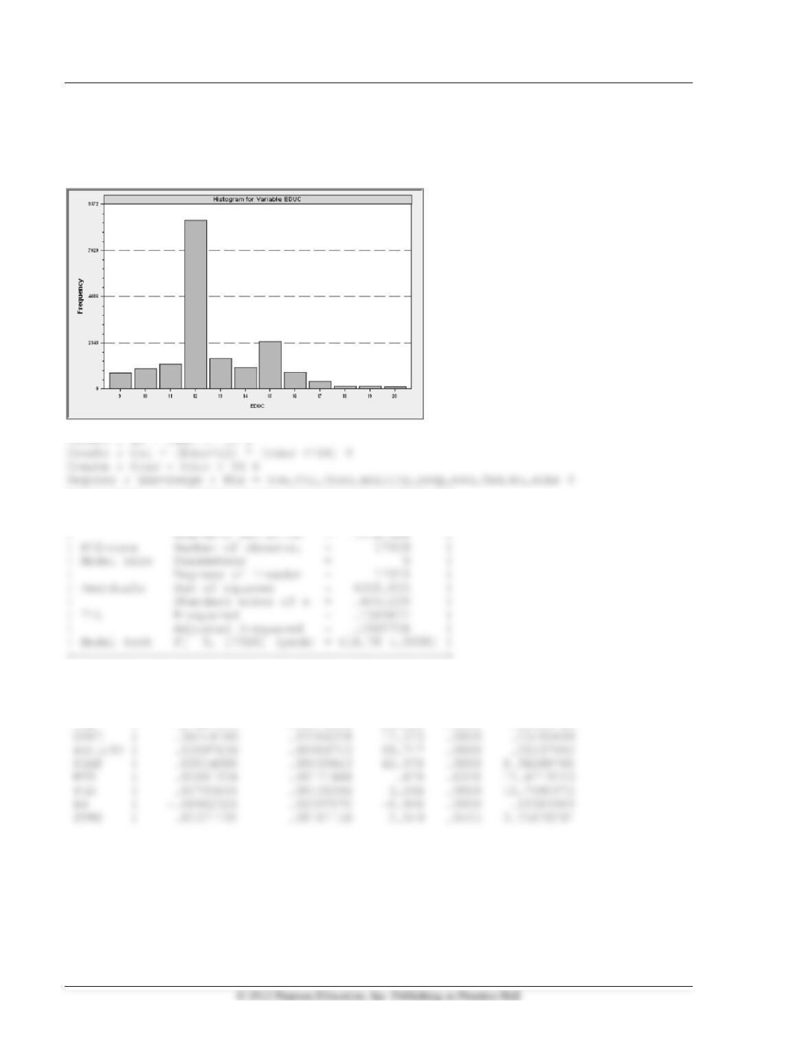
Histogram ; Rhs = Educ $
+—————————————————-+
| Ordinary least squares regression |
| LHS=LWAGE Mean = 2.296821 |
+——–+————–+—————-+——–+——–+———-+
|Variable| Coefficient | Standard Error |b/St.Er.|P[|Z|>z]| Mean of X|
+——–+————–+—————-+——–+——–+———-+
Constant| 1.81124933 .02069456 87.523 .0000
COL | .17467913 .00872506 20.020 .0000 .32183716
Chapter 6 Functional Form and Structural Change 43
c. Education squared
Create ; educsq = educ*educ $
Regress ; Lhs = lwage;rhs=one,educ,educsq,ability,pexp,med,fed,bh,sibs$
+—————————————————-+
| Ordinary least squares regression |
| LHS=LWAGE Mean = 2.296821 |
| Standard deviation = .5282364 |
+—————————————————-+
+——–+————–+—————-+——–+——–+———-+
|Variable| Coefficient | Standard Error |b/St.Er.|P[|Z|>z]| Mean of X|
+——–+————–+—————-+——–+——–+———-+
Constant| .42778242 .12008093 3.562 .0004
EDUC | .15590624 .01751608 8.901 .0000 12.6760422
44 Greene • Econometric Analysis, Seventh Edition
d. Interaction
Sample ; All $
+—————————————————-+
| Ordinary least squares regression |
| LHS=LWAGE Mean = 2.296821 |
+—————————————————-+
+——–+————–+—————-+——–+——–+———-+
|Variable| Coefficient | Standard Error |b/St.Er.|P[|Z|>z]| Mean of X|
+——–+————–+—————-+——–+——–+———-+
Constant| 1.00190276 .03529335 28.388 .0000
EDUC | .07006221 .00243183 28.811 .0000 12.6760422
+————————————+
| Listed Calculator Results |
+————————————+
ME = .070195
e.
Regress ; Lhs = lwage;rhs=one,educ,educsq,ability,ea,pexp,med,fed,bh,sibs$
+—————————————————-+
| Ordinary least squares regression |
| LHS=LWAGE Mean = 2.296821 |
| Standard deviation = .5282364 |
Chapter 6 Functional Form and Structural Change 45
+——–+————–+—————-+——–+——–+———-+
|Variable| Coefficient | Standard Error |b/St.Er.|P[|Z|>z]| Mean of X|
+——–+————–+—————-+——–+——–+———-+
Constant| -.10514525 .14931731 -.704 .4813
EDUC | .24088793 .02252126 10.696 .0000 12.6760422
+————————————+
| Listed Calculator Results |
+————————————+
AVGLOW = -.798563
46 Greene • Econometric Analysis, Seventh Edition
?=======================================================================
? Application 6.2
?=======================================================================
Sample ; All $
Namelist ; X = one,educ,ability,pexp,med,fed,sibs$
+————————————+
| Listed Calculator Results |
+————————————+
CHOW = 7.348379
1
?=======================================================================
a. The least squares estimates of the four models are
q/A = 0.45237 + 0.23815lnk
q/A = 0.91967 − 0.61863/k
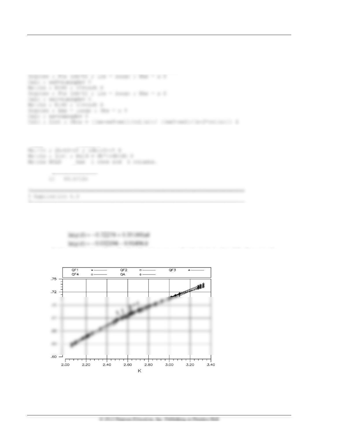
At these parameter values, the four functions are nearly identical. A plot of the four sets of
predictions from the regressions and the actual values appears below.
Chapter 6 Functional Form and Structural Change 47
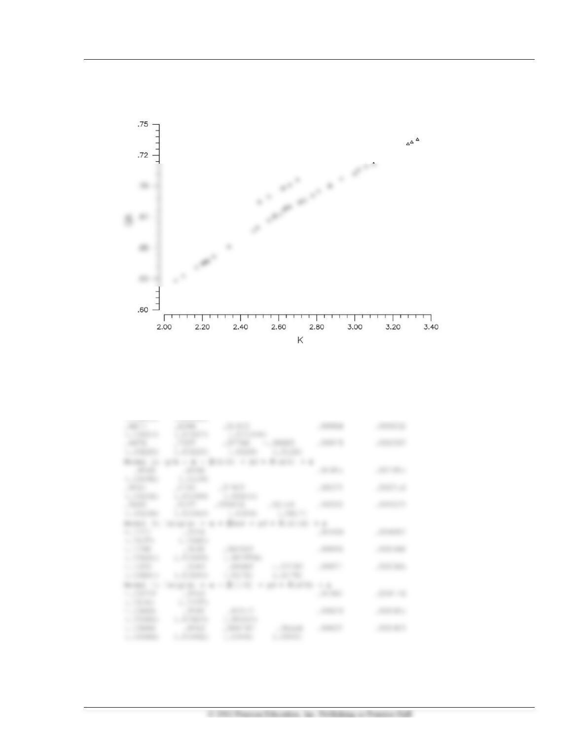
b. The scatter diagram is shown below. The last seven years of the data set show clearly the effect
observed by Solow.
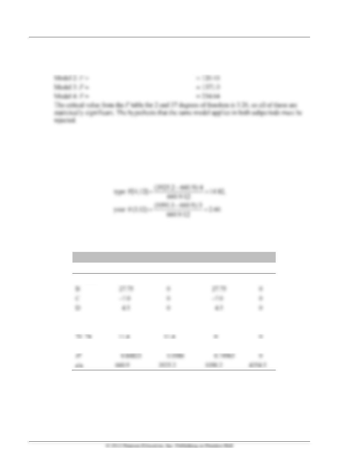
c. The regression results for the various models are listed below. (d is the dummy variable equal
to 1 for the last seven years of the data set. Standard errors for parameter estimates are given
in parentheses.)
R2 ee
Model 1:q/A = + lnk + d + (dlnk) +
.4524 .2381 .94355 .00213
(.00903) (.00932)
48 Greene • Econometric Analysis, Seventh Edition
d. For the four models, the F test of the third specification against the first is equivalent to the
Chow-test. The statistics are:
Model 1: F = (0.002126 − 0.000032)/2/(0.000032/37) = 1210.6
?=======================================================================
? Application 6.4
?=======================================================================
According to the full model, the expected number of incidents for a ship of the base type A built
in the base period 1960 to 1964, is 3.4. The other 19 predicted values follow from the previous
results and are left as an exercise. The relevant test statistics for differences across ship type and
year are as follows:
The 5 percent critical values from the F table with these degrees of freedom are 3.26 and 3.49,
respectively, so we would conclude that the average number of incidents varies significantly
across ship types but not across years.
Regression Coefficients
Full Model
Time Effects
Type Effects
No Effects
Constant
3.4
6.0
8.25
10.85
B
0
27.75
0
C
0
0
D
0
0
E
–3.25
0
–3.25
0
65–69
7.0
7.0
0
0
70–74
11.4
0
0
75–79
1.0
1.0
0
0
0