132 Abel/Bernanke/Croushore • Macroeconomics, Ninth Edition
◼ Answers to Textbook Problems
Review Questions
1. The three sources of economic growth are capital growth, labor growth, and productivity growth. The
growth accounting approach is derived from the production function.
2. A decline in productivity growth is the primary reason for the slowdown in output growth in the
3. The rise in productivity growth in the 1990s occurred because of the revolution in information and
communications technologies (ICT). Not only were there improvements in ICT, but also government
4. A steady state is a situation in which the economy’s output per worker, consumption per worker,
and capital stock per worker are constant.
6. The statement is false. Increases in the capital-labor ratio increase consumption per worker in the
7. (a) An increase in the saving rate increases long-run living standards, as higher saving allows for
more investment and a larger capital stock.
8. Endogenous growth theory suggests that the main sources of productivity growth are accumulation
of human capital (the knowledge, skills, and training of individuals) and technological innovation
9. Government policies to promote economic growth include policies to raise the saving rate and
policies to increase productivity. One way to increase the saving rate is to increase the real return
to saving by providing a tax break, as Individual Retirement Accounts did in the United States.
Unfortunately, the response of saving to increases in the real rate of return is small. Another way to
increase the saving rate is to reduce the government budget deficit. However, the theory of Ricardian
Chapter 6 Long-Run Economic Growth 133
One way that government policy can increase productivity is by spending more on the economy’s
infrastructure, which has been neglected over the past two decades in the United States. Another
possibility is to support the creation of human capital by spending more on education and training
programs, and reducing barriers to entrepreneurial activity. The issue is whether the government
134 Abel/Bernanke/Croushore • Macroeconomics, Ninth Edition
Numerical Problems
1. Hare: $5000 (1.03)70 = $39,589
Tortoise: $5000 (1.01)70 = $10,034
2.
20 Years Ago
Today
Percent Change
Y
1000
1300
30%
K
2500
3250
30%
(b) A/A = 30% − (0.5 30%) − (0.5 15%)
= 30% − 15% − 7.5%
= 7.5%
Capital growth contributed 15% (aK K/K), labor growth contributed 7.5% (aN N/N),
productivity growth was 7.5%.
3. (a)
Year
K
N
Y
K/N
Y/N
1
200
1000
617
0.20
0.617
3
250
1250
0.617
(b)
Year
K
N
Y
K/N
Y/N
1
200
1000
1231
0.20
1.231
2
250
1000
1316
0.25
1.316
3
250
1250
1574
0.20
1.259
Chapter 6 Long-Run Economic Growth 135
4. To answer this problem, an approximate solution can be found by finding the ratio GDP (2010)/GDP
(1950), taking the natural logarithm of that ratio and dividing by 60. This is the answer given in the
table below.
Real GDP Per Capita
Growth
1950
2010
Ratio
Rate
Australia
7,412
25,301
3.41
2.1%
Canada
7,291
25,267
3.47
2.1%
France
5,186
22,223
4.29
2.5%
Germany
3,881
20,801
5.36
2.9%
Sweden
6,769
24,409
3.61
2.2%
United Kingdom
6,939
23,742
3.42
2.1%
United States
9,561
31,178
3.26
2.0%
5. (a) sf(k) = (n + d)k
0.3 3k.5 = (0.05 + 0.1)k
0.9k.5 = 0.15k
0.9/0.15 = k/k.5
136 Abel/Bernanke/Croushore • Macroeconomics, Ninth Edition
(d) sf(k) = (n + d)k
0.3 4k.5 = (0.05 + 0.1)k
6. (a) In steady state, sf(k) = (n + d)k
0.1 6k.5 = (0.01 + 0.14)k
(b) To get y = 2 24 = 48, since y = 6k.5, then 48 = 6k.5, so k.5 = 8, so k = 64. The capital-labor ratio
would need to increase from 16 to 64. To get k = 64, since sf(k) = (n + d)k, s 48 = 0.15 64, so
s = 0.2. Saving per worker would need to double.
7. First, derive saving per worker as sy = y − c − g = [1 − 0.5(1 − t) − t] 8k.5 = 0.5(1 − t)8k.5 = 4 (1 − t)k.5
(a) When t = 0, sy = 4 (1 − 0)k.5 = 4k.5 = national saving per worker
Investment per worker = (n + d)k = 0.1k
In steady state, sy = (n + d)k, so 4k.5 = 0.1k, or 40k.5 = k, so 1600k = k2, so k = 1600. Since k = 1600,
Chapter 6 Long-Run Economic Growth 137
Analytical Problems
1. (a) The destruction of some of a country’s capital stock in a war would have no effect on the steady
state, because there has been no change in s, f, n, or d. Instead, k is reduced temporarily, but
equilibrium forces eventually drive k to the same steady-state value as before.
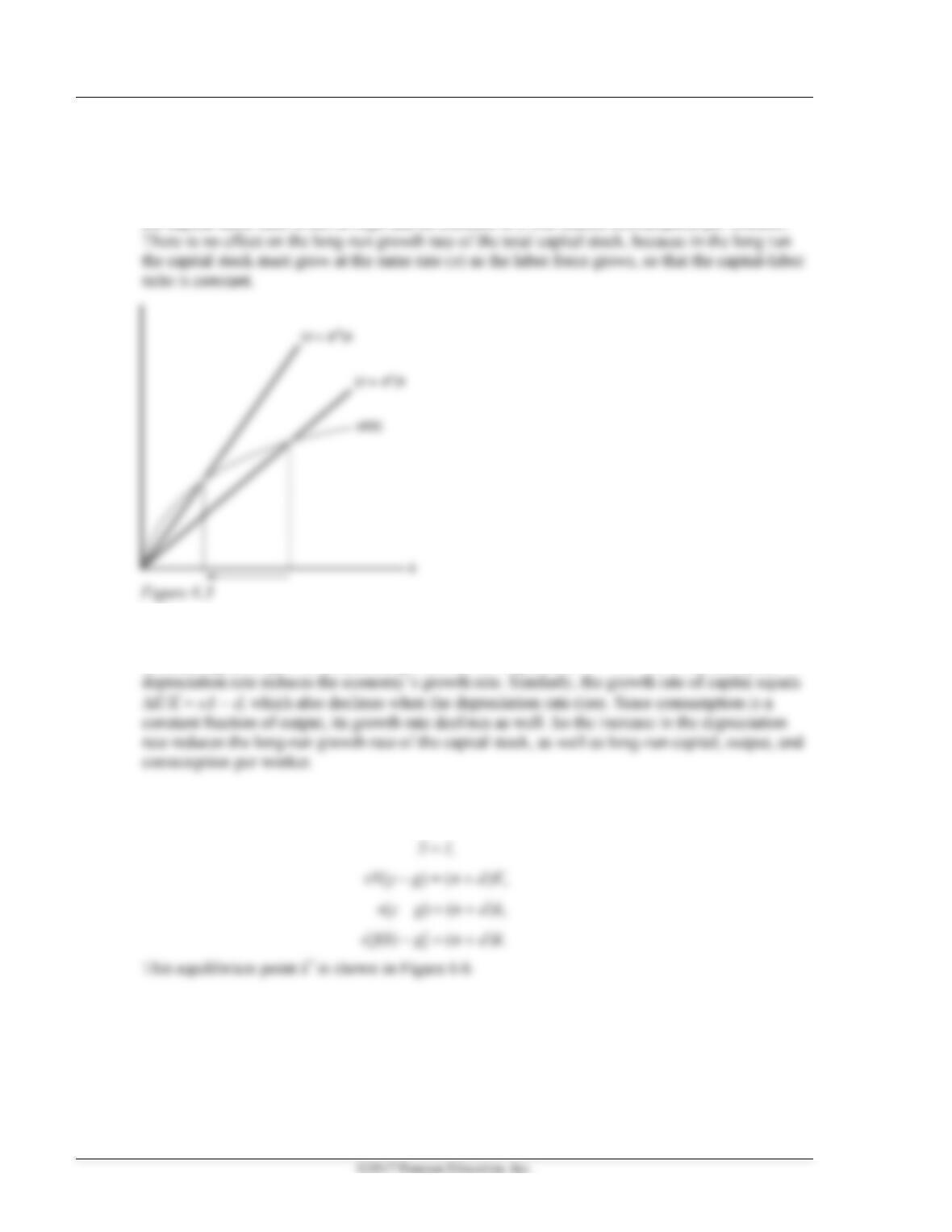
(b) Immigration raises n from n1 to n2 in Figure 6.3. The rise in n lowers steady-state k, leading to a
lower steady-state consumption per worker.
(c) The rise in energy prices reduces the productivity of capital per worker. This causes sf(k) to shift
down from sf 1(k) to sf 2(k) in Figure 6.4. The result is a decline in steady-state k. Steady-state
138 Abel/Bernanke/Croushore • Macroeconomics, Ninth Edition
2. (a) Solow model
The rise in capital depreciation shifts up the (n + d)k line from (n + d1)k to (n + d2)k, as shown in
Figure 6.5. The equilibrium steady-state capital-labor ratio declines. With a lower capital-labor
ratio, output per worker is lower, so consumption per worker is lower (using the assumption that
the capital-labor ratio is not so high that an increase in k will reduce consumption per worker).
(b) Endogenous growth model
In an endogenous growth model, the growth rate of output is Y/Y = sA − d, so the rise in the
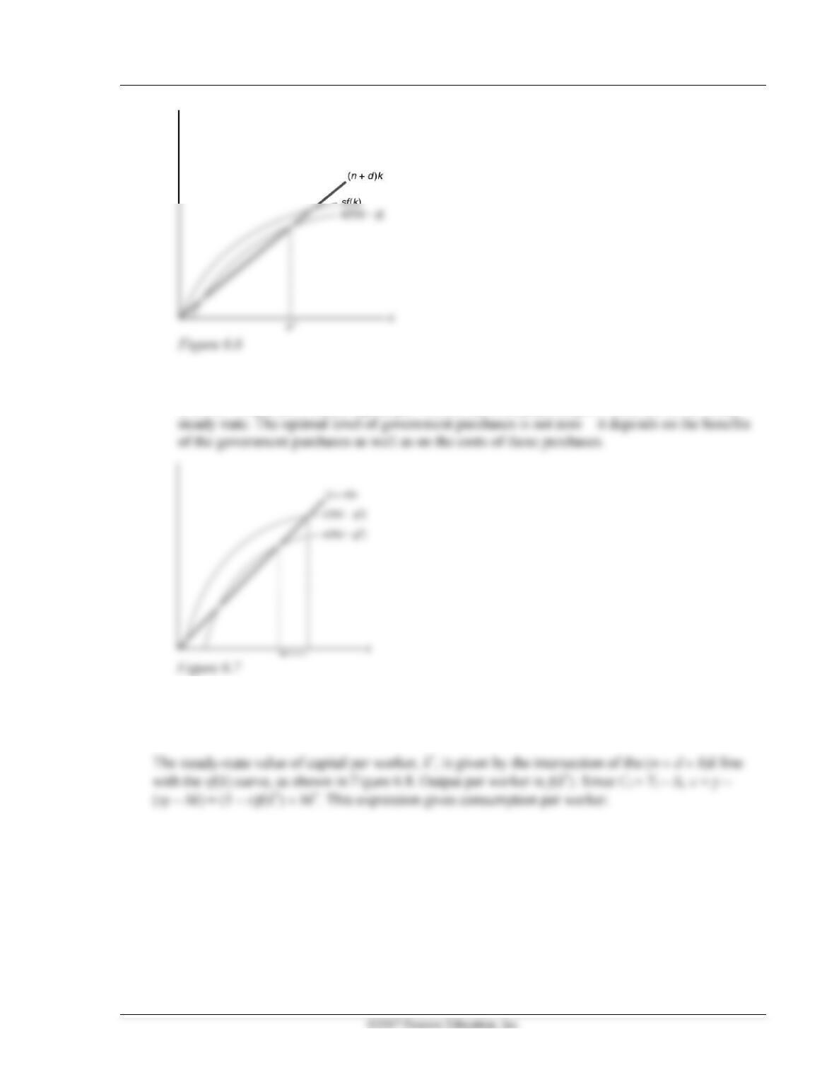
3. (a) With a balanced budget T/N = g. National saving is S = s(Y – T) = sN[(Y/N) − (T/N)] =
sN(y – g). Setting saving equal to investment gives
Chapter 6 Long-Run Economic Growth 139
(b) If the government permanently increases purchases per worker, the s[f(k) – g] curve shifts down
from s[f(k) – g1] to s[f(k) – g2] in Figure 6.7. In steady-state equilibrium, the capital-labor ratio
is lower. Output per worker, capital per worker, and consumption per worker are lower in the
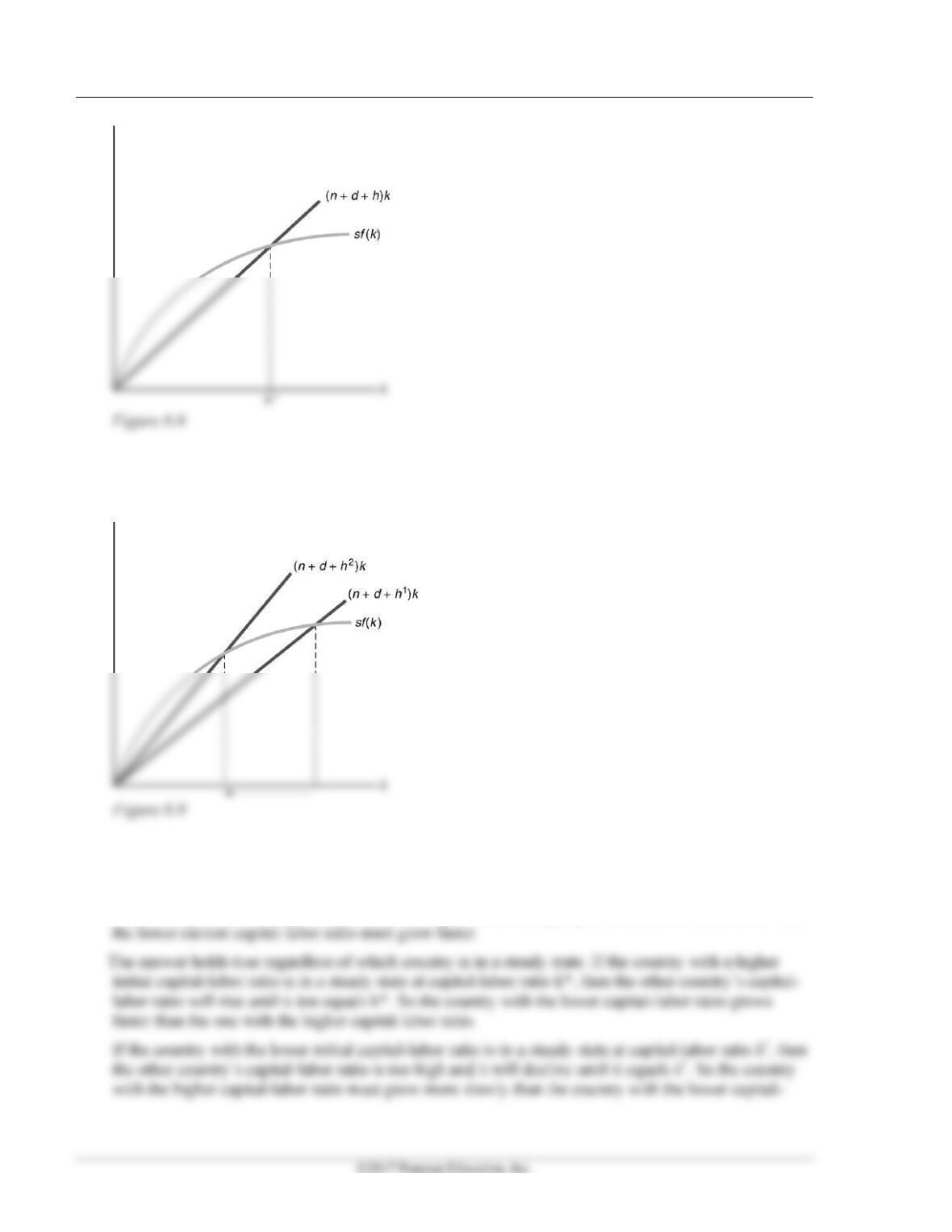
4. St = sYt – hKt = Nt(syt – hkt). Setting St = It yields Nt(syt – hkt) = (n + d)Kt. Dividing through by Nt and
eliminating time subscripts for steady-state variables gives sy – hk = (n + d)k. Rearranging and using
the expression y = f(k) gives sf(k) = (n + d + h)k.
140 Abel/Bernanke/Croushore • Macroeconomics, Ninth Edition
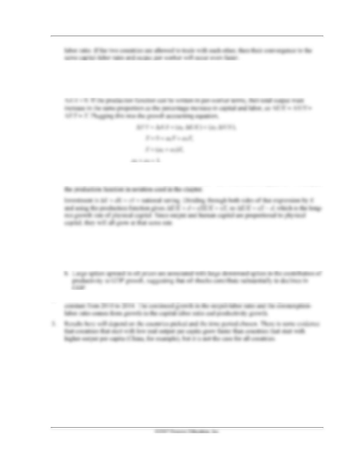
A change in the steady-state value of h increases the slope of the (n + d + h)k line, as shown in
Figure 6.9. This reduces the steady-state value of per-worker capital (k*), per-worker output
[since y* = f(k*)], and per-worker consumption [since c* = (1 − s)y* + hk* and both y* and k* decline].
5. The initial level of the capital-labor ratio is irrelevant for the steady state. Two economies that are
identical except for their initial capital-labor ratios will have exactly the same steady state.
Since the two economies must have the same growth rate at the steady state, and since the economy
with the higher current capital-labor ratio has higher current output per worker, then the country with
Chapter 6 Long-Run Economic Growth 141
6. The growth accounting equation is
Y/Y = A/A + (aK K/K) + (aN N/N).
We are just increasing the amount of capital and labor, and there is no change in productivity, so
7. Assume there are a constant number of workers, N, so that Ny = Y and Nk
=
K. Since y = Akah1–a and
h = Bk, then y = Aka(Bk)1–a = (AB1–a)k. Then Y = Ny = (AB1–a)K = XK, where X equals AB1–a. This puts
Working with Macroeconomic Data
1. a. After 1973, productivity contributes less to GDP growth than before 1973. Productivity’s
contribution declines sharply in the 1970s and early 1980s.
2. There is little evidence of a steady state being reached in the capital-labor ratio, though it is fairly