Demand Estimation 121
P5.5 Linear Demand Curve Estimation. Xerox Corporation develops, manufactures, and
services document equipment and software solutions worldwide. Assume the company
offered $75 off the $1,475 regular price on the Phaser 6360, a durable high-speed color
copier, and Internet sales jumped from 700 to 800 units per week (see
http://www.office.xerox.com).
A. Estimate the color copier demand curve, assuming that it is linear.
B. If marginal costs per unit are $650, calculate the profit-maximizing price/output
combination. [Remember: The marginal revenue curve has the same intercept as
the demand curve, but has twice its negative slope (falls twice as fast).]
P5.5 SOLUTION
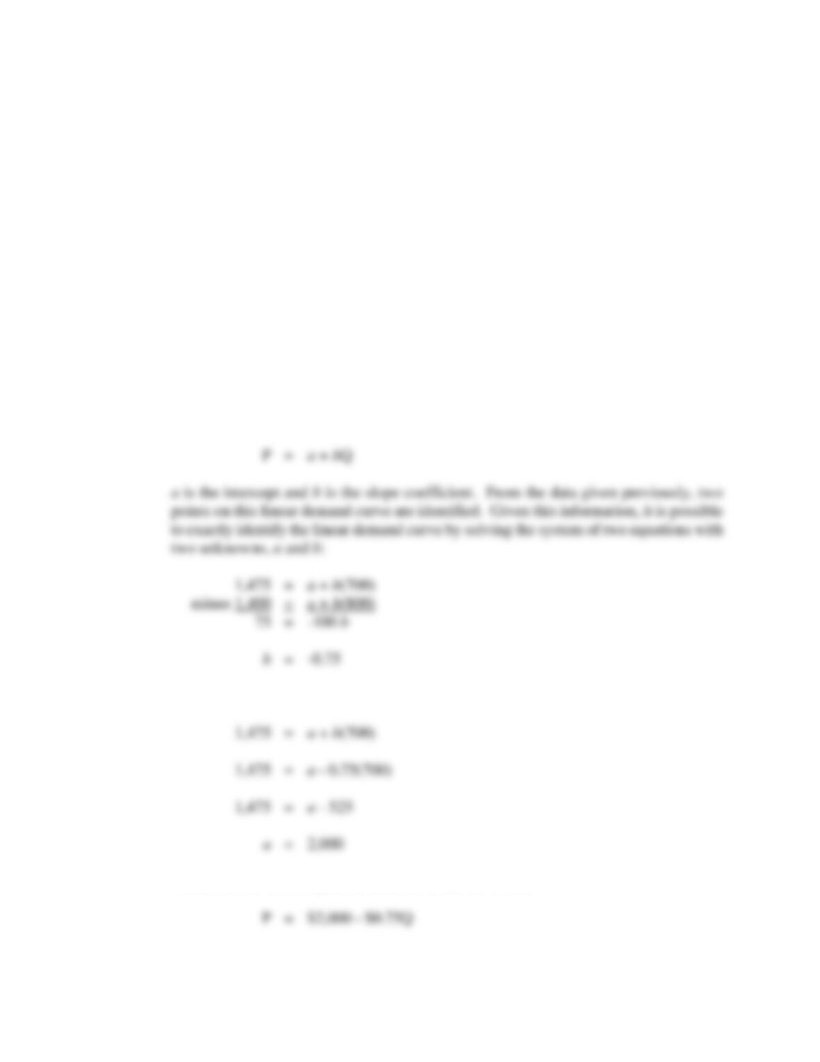
A. When a linear demand curve is written as:
By substitution, if b = -0.75, then:
Therefore, the color copier demand curve can be written:
122 Chapter 5
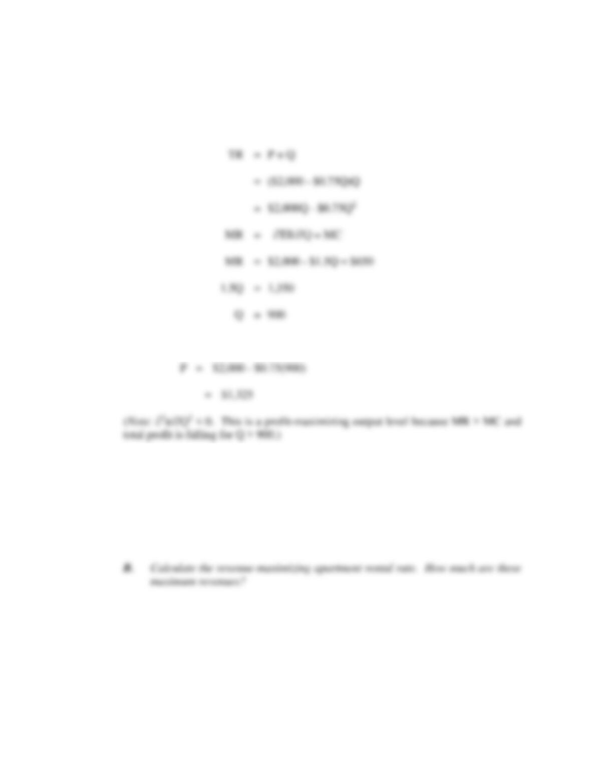
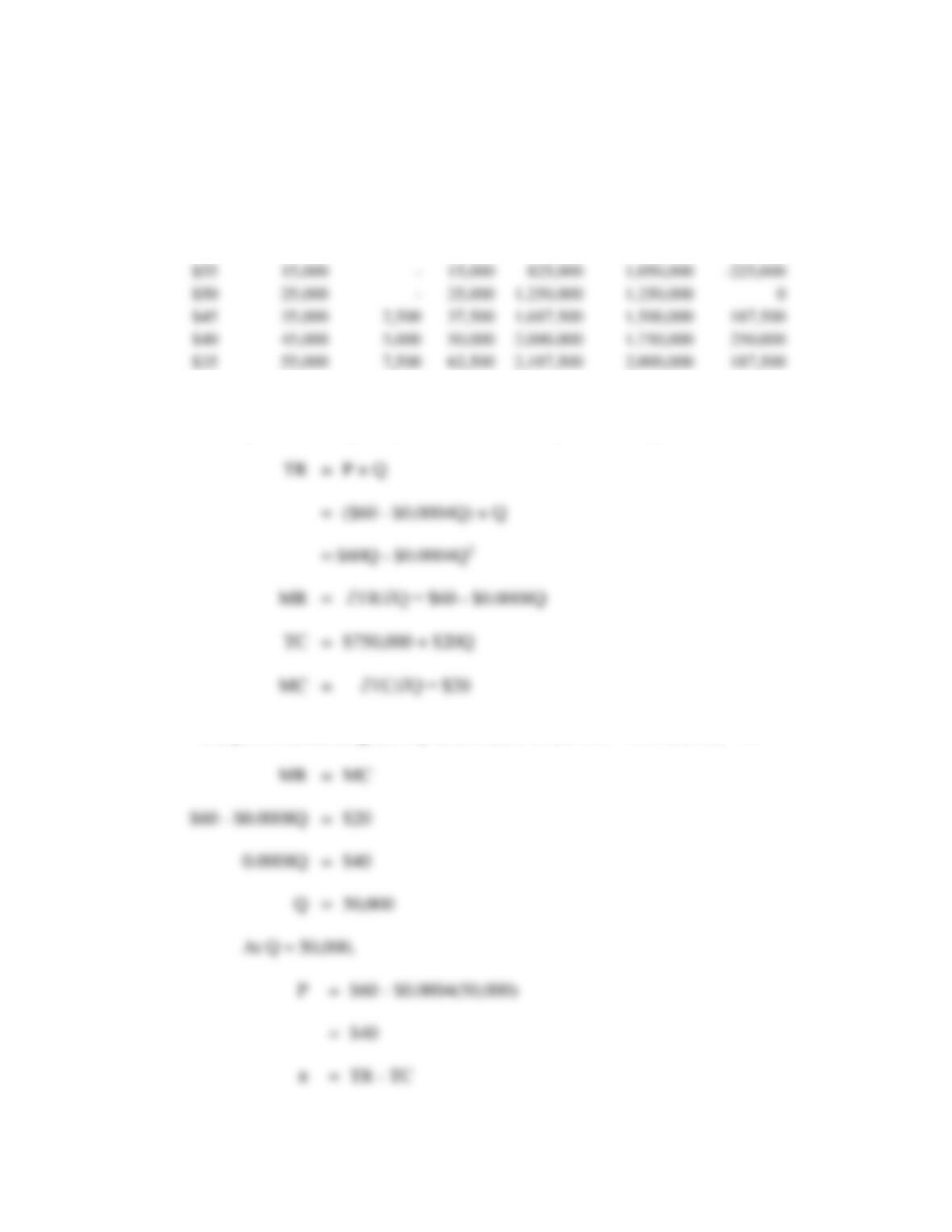
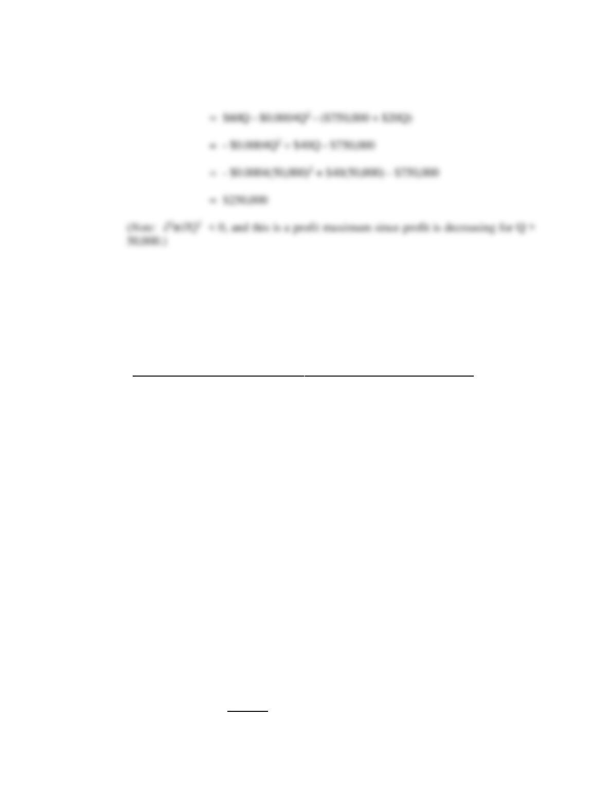
B. To find the profit-maximizing output level, set MR = $650 = MC, and solve for Q.
Because
At Q = 900, the profit-maximizing price is
P5.6 Linear Demand Curve Estimation. Kenny McCormick manages a 100-unit apartment
building and knows from experience that all units will be occupied if rent is $900 per
month. McCormick also knows that, on average, one additional unit will go unoccupied
for each $10 increase in the monthly rental rate.
A. Estimate the apartment rental demand curve assuming that it is linear and that
price is expressed as a function of output.
C. If all costs are fixed, what is the profit-maximizing number of vacant apartments?
Explain your answer.
P5.6 SOLUTION
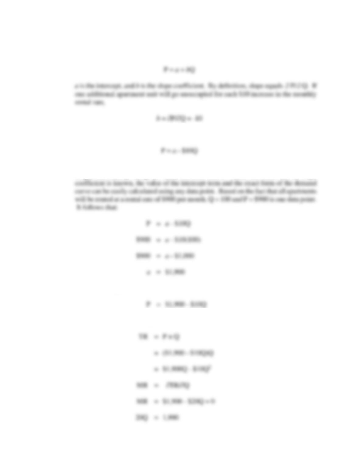
A. When a linear demand curve is written as:
Demand Estimation 123
Therefore,
Under the assumption of a linear demand relation, each of the data points for price and
output fall exactly along the linear demand curve. Once the value of the slope
Therefore, in general:
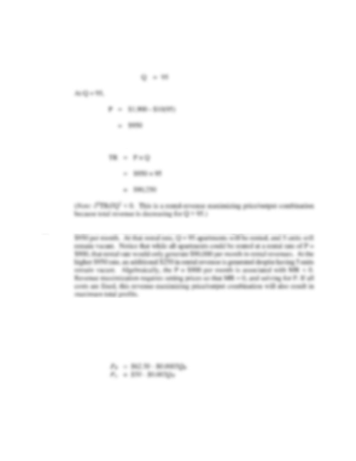
B. To find the revenue-maximizing rental rate, set MR = 0, and solve for P. Because
124 Chapter 5
Total revenue at a price of $950 is:
C. In part B, it was determined that the revenue-maximizing apartment rental rate is P =
P5.7 Market Demand. Gregory House, a Philadelphia-based management consultant, has
been asked to calculate and analyze market demand for a new video game that is to be
marketed to retail (R) and wholesale (W) customers over the Internet.
The client estimates fixed costs of $750,000 per year for the product, and that
licensing fees and other marginal costs will be $20 per unit. The client has also
provided the following annual demand information:
A. Express quantity as a function of price for both retail and wholesale customers.
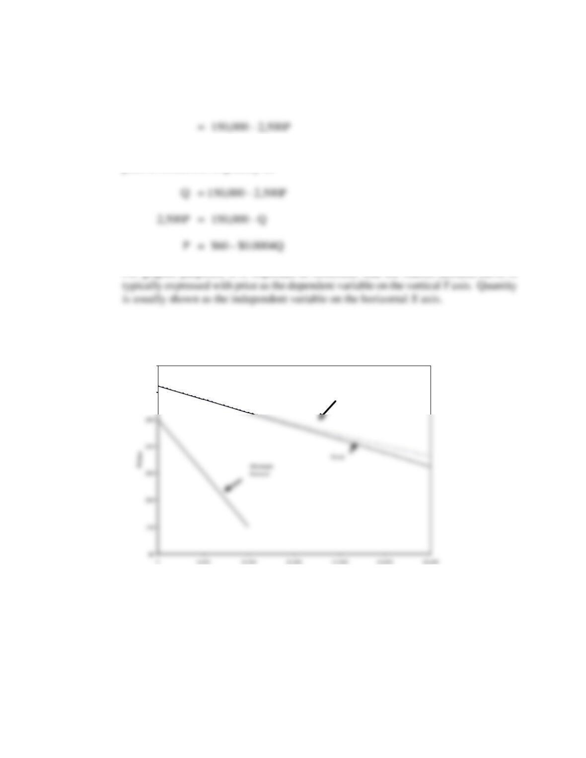
Add these quantities together to calculate the market demand curve. Graph the
retail, wholesale, and market demand curves for prices ranging from $65 to $35
per unit.
Demand Estimation 125
Market Demand is Retail Plus Wholesale Demand
Price
Retail
Demand
Wholesale
Demand
Market
Demand
Total
Revenue
Total Cost
Total Profit
$65
$60
$50
$35
P5.7 SOLUTION
A. To find the market demand curve, it is necessary to express quantity as a function of
price for both retail and wholesale customers. Then, these quantities must be added
For wholesale customers,
For retail plus wholesale customers, the market demand curve can be expressed with
quantity as a function of price as:
126 Chapter 5
For retail plus wholesale customers, the market demand curve can be expressed with
price as a function of quantity as:
For graphic purposes, it is important to remember that the market demand curve is
B.
Market Demand is Retail Plus Wholesale Demand
Market Dem and is Retail Plus Wholesale Demand
$60
$70
Qua nt i t y
Mar ket Demand
Demand Estimation 127
Price
Retail
Demand
Wholesale
Demand
Market
Demand
Total
Revenue
Total Cost
Total Profit
$65
–
–
–
–
750,000
-750,000
$60
5,000
–
5,000
300,000
850,000
-550,000
$55
15,000
–
15,000
825,000
1,050,000
-225,000
C. From the table, the profit-maximizing activity level can be seen as the $40 price and 50,000
unit activity level. Analytically, this can be found by first solving for MR and MC,
The profit-maximizing activity level occurs where MR = MC, and Mπ = 0.
$45
35,000
37,500
1,687,500
1,500,000
$40
45,000
50,000
2,000,000
1,750,000
$35
55,000
62,500
2,187,500
2,000,000
128 Chapter 5
P5.8 Identification Problem. Business is booming for Consulting Services, Inc. (CSI), a local
supplier of computer set-up consulting services. The company can profitably employ
technicians as quickly as they can be trained. The average hourly rate billed by CSI for
trained technician services and the number of billable hours (output) per quarter over
the past six quarters are as follows:
Q-1
Q-2
Q-3
Q-4
Q-5
Q-6
Hourly rate ($)
$20
$25
$30
$35
$40
$45
Billable hours
2,000
3,000
4,000
5,000
6,000
7,000
Quarterly demand and supply curves for CSI services are
QD = 4,000 – 200P + 2,000T (Demand),
QS = -2,000 + 200P (Supply),
where Q is output, P is price, T is a trend factor, and T = 1 during Q-1 and increases by
one unit per quarter.
A. Express each demand and supply curve in terms of price as a function of output.
B. Plot the quarterly demand curves for the last six quarterly periods. (Hint: Let T
= 1 to find the Y intercept for Q-1, T = 2 for Q-2, and so on.)
C. Plot the CSI supply curve on the same graph.
D. What is this problem’s relation to the identification problem?
P5.8 SOLUTION
A. Demand
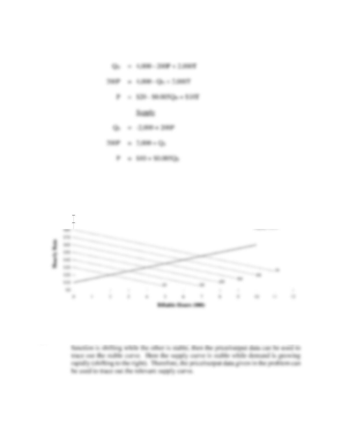
Demand Estimation 129
B.,C.
D. This problem illustrates the identification problem. If either the demand or supply
P5.9 Multiple Regression. Colorful Tile, Inc., is a rapidly growing chain of ceramic tile
outlets that caters to the do–it-yourself home remodeling market. In 2007, 33 stores
Consulting Services, Inc., Demand and Supply Curve Analysis
$90
$100
Supply Curve
130 Chapter 5
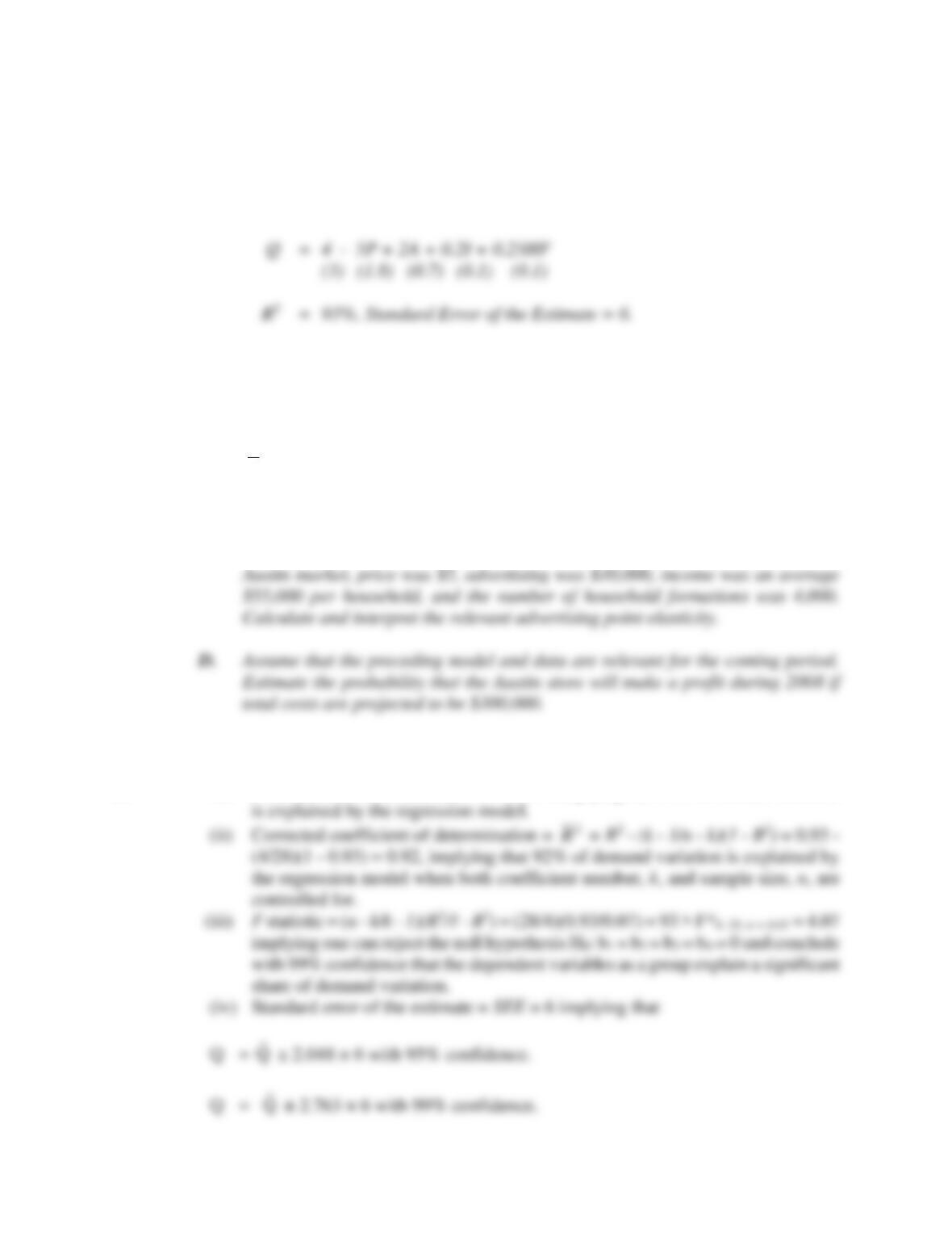
were operated in small to medium-size metropolitan markets. An in-house study of sales
by these outlets revealed the following (standard errors in parentheses):
Here, Q is tile sales (in thousands of cases), P is tile price (per case), A is advertising
expenditures (in thousands of dollars), I is disposable income per household (in
thousands of dollars), and HF is household formation (in hundreds).
A. Fully evaluate and interpret these empirical results on an overall basis using R2,
2
R
, F-statistic and SEE information.
B. Is quantity demanded sensitive to “own” price?
C. Austin, Texas, was a typical market covered by this analysis. During 2007 in the
P5.9 SOLUTION
A. (i) Coefficient of determination = R2 = 93%, implying that 93% of demand variation
2
R
Demand Estimation 131
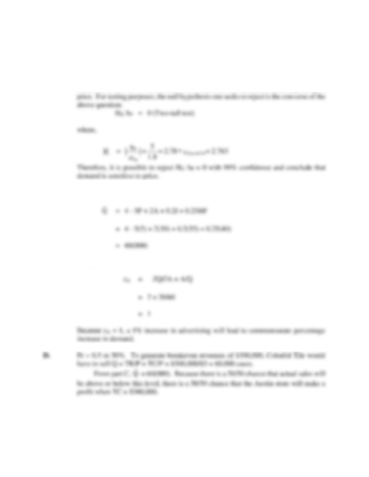
B. To determine whether quantity demanded depends upon “own” price, the question must
be asked: is bP ≠ 0? If bP ≠ 0, then evidence exists that sales do indeed depend upon
C. Because
The point advertising elasticity is calculated as:
P5.10 Multiplicative Demand Functions. Getaway Tours, Inc., has estimated the following
multiplicative demand function for packaged holiday tours in the East Lansing,
Michigan, market using quarterly data covering the past four years (16 observations):
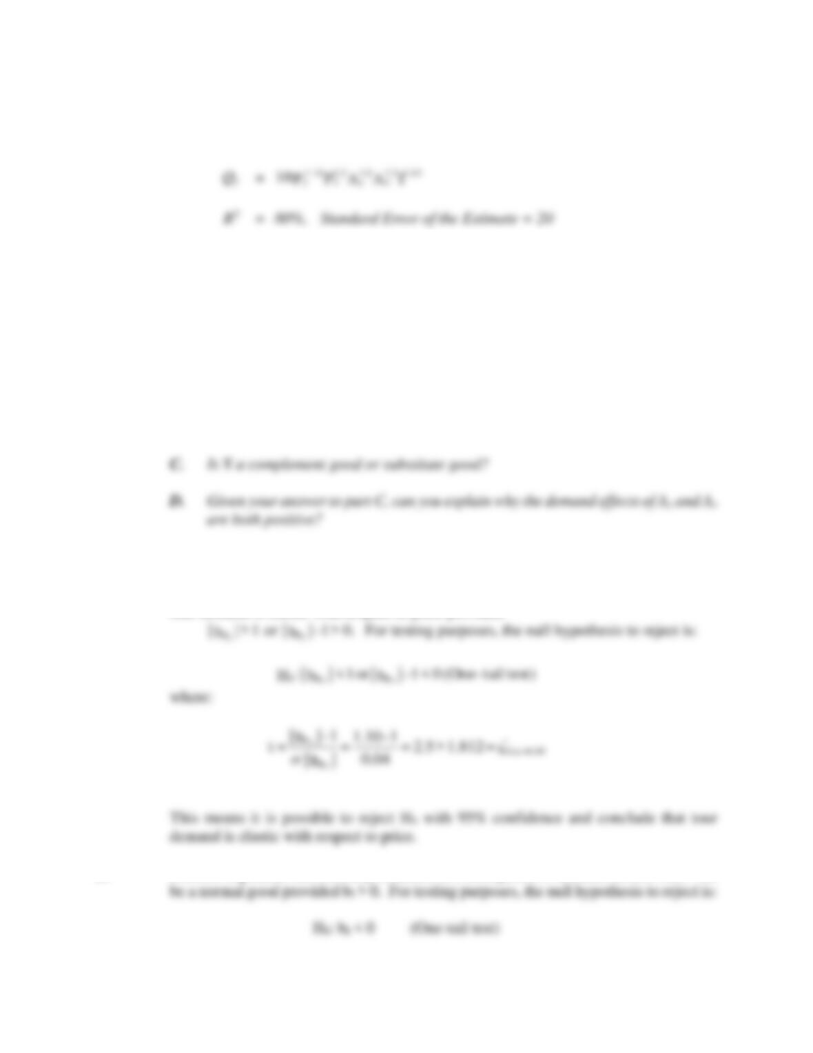
132 Chapter 5
Here, Qy is the quantity of tours sold, Py is average tour price, Px is average price for
some other good, Ay is tour advertising, Ax is advertising of some other good, and I is
per capita disposable income. The standard errors of the exponents in the preceding
multiplicative demand function are
A. Is tour demand elastic with respect to price?
B. Are tours a normal good?
P5.10 SOLUTION
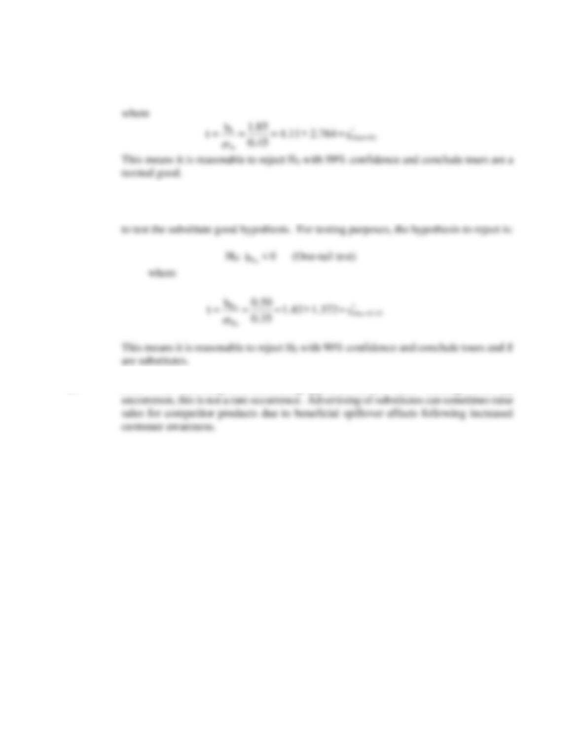
A. The exponents of multiplicative demand functions are elasticity estimates. Therefore,
tour demand is elastic with respect to price provided
B. Because exponents are elasticity estimates in a multiplicative demand model, tours will
0.45. =
b
and 0.9, =
b
0.5, =
b
0.35, =
b
0.04, =
bI
AAPP xyxy
Demand Estimation 133
C. Because exponents are elasticity estimates in a multiplicative demand model, tours and
X will be substitutes provided
0, >
bPX
and complements if
0. <
bPX
One may first wish
D. Both “own” and competitor advertising appear to increase sales. Although relatively
134 Chapter 5
CASE STUDY FOR CHAPTER 5
Demand Estimation for Mrs. Smyth’s Pies
Demand estimation for brand-name consumer products is made difficult by the fact that managers
To see the process that might be undertaken to develop a better understanding of product
demand conditions, consider the hypothetical example of Mrs. Smyth’s Inc., a Chicago-based food
company. In early 2008, Mrs. Smyth’s initiated an empirical estimation of demand for its gourmet
frozen fruit pies. The firm is formulating pricing and promotional plans for the coming year, and
management is interested in learning how pricing and promotional decisions might affect sales.
The following regression equation was fit to these data:
Q is the quantity of pies sold during the tth quarter; P is the retail price in dollars of Mrs. Smyth’s
frozen pies; A represents the dollars spent for advertising; PX is the price, measured in dollars,
charged for competing premium-quality frozen fruit pies; Y is the median dollars of disposable
A. Describe the economic meaning and statistical significance of each individual
independent variable included in the Mrs. Smyth’s frozen fruit pie demand equation.
B. Interpret the coefficient of determination (R2) for the Mrs. Smyth’s frozen fruit pie
demand equation.
Demand Estimation 135
C. Use the regression model and 2007-4 data to estimate 2008-1 unit sales in the
Washington-Arlington-Alexandria market.
CASE STUDY SOLUTION
A. The individual coefficients for the Mrs. Smyth’s pie demand regression equation can be
interpreted as follows. The intercept term, 529,774, has no economic meaning in this
instance; it lies far outside the range of observed data and obviously cannot be
Individual coefficients provide useful estimates of the expected marginal influence
on demand following a one-unit change in each respective variable. However, they are
only estimates. For example, it would be very unusual for a $1 increase in price to cause
exactly a -122,607-unit change in the quantity demanded. The actual effect could be
more or less. For decision-making purposes, it would be helpful to know if the marginal
influences suggested by the regression model are stable or instead tend to vary widely
136 Chapter 5
B. The coefficient of determination R2 = 0.871 or 87.1 percent indicates that the regression
model has explained 87.1 percent of the total variation in pie demand. This is a very
satisfactory level of explanation for the model as a whole. The corrected coefficient of
C. To project the next quarter’s sales of frozen fruit pies in the Washington, DC-Arlington-
Alexandria market, the company must simply enter expected values for each
independent variable in the estimated demand equation. Mrs. Smyth’s expects an
average price for its pies of $7.95, advertising expenditures of $30,487. The prices of
Demand Estimation 137
D. Although 200,430 is the best estimate of pie demand for the Washington, DC-Arlington-
Alexandria market during the 2008-1 period, it is highly unlikely that precisely this number
of pies will be sold. Either more or less may be sold, depending on the effects of other