Basic Econometrics, Gujarati and Porter
33
CHAPTER 5:
TWO-VARIABLE REGRESSION:
INTERVAL ESTIMATION AND HYPOTHESIS TESTING
Questions
5.1 (a) True. The t test is based on variables with a normal distribution.
34
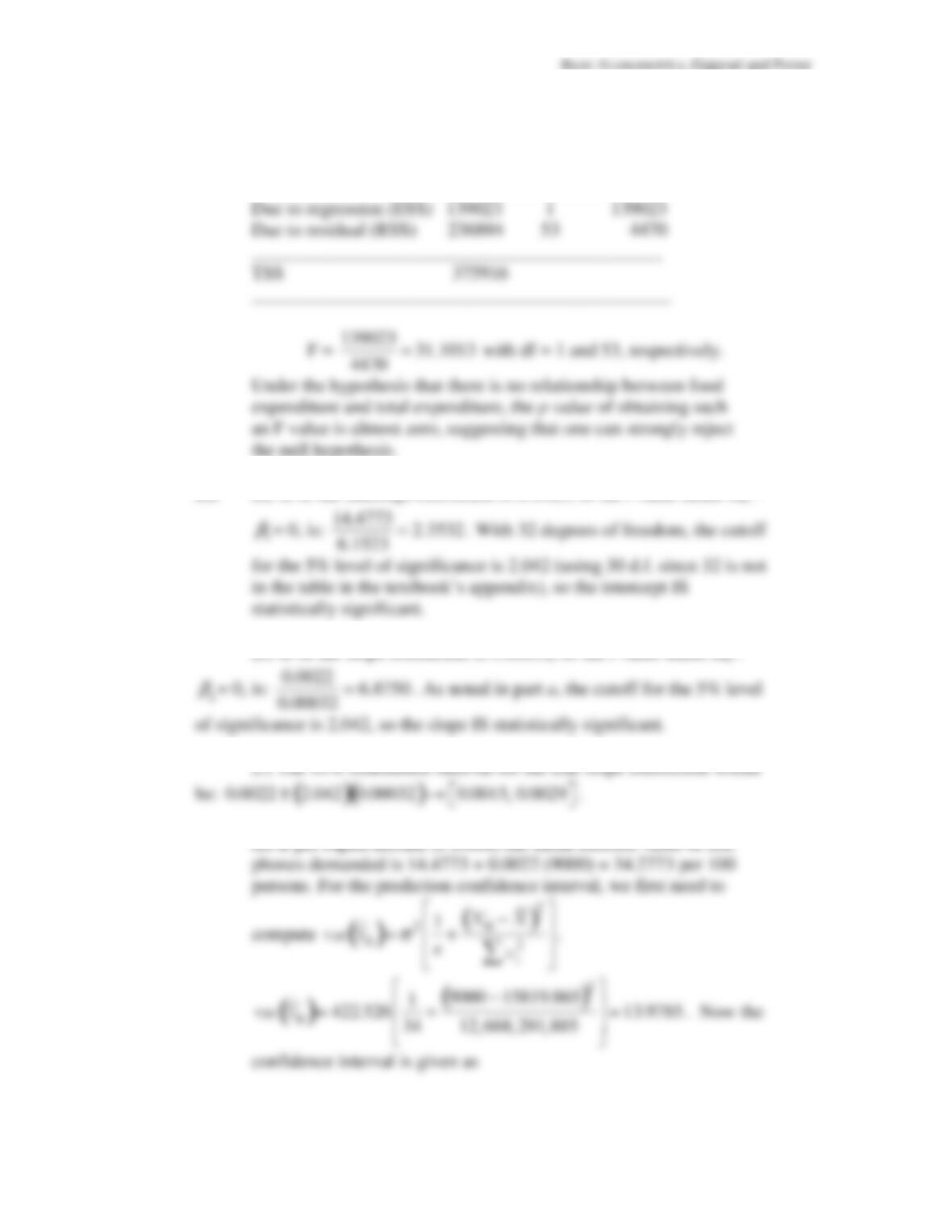
5.2
ANOVA table for the Food Expenditure in India
__________________________________________
Source of variation SS df MSS
__________________________________________
5.3
(
a
) se of the intercept coefficient is 6.1523, so the
t
value under H
:
(
b
) se of the slope coefficient is 0.00032, so the
t
value under H
:
Basic Econometrics, Gujarati and Porter
35
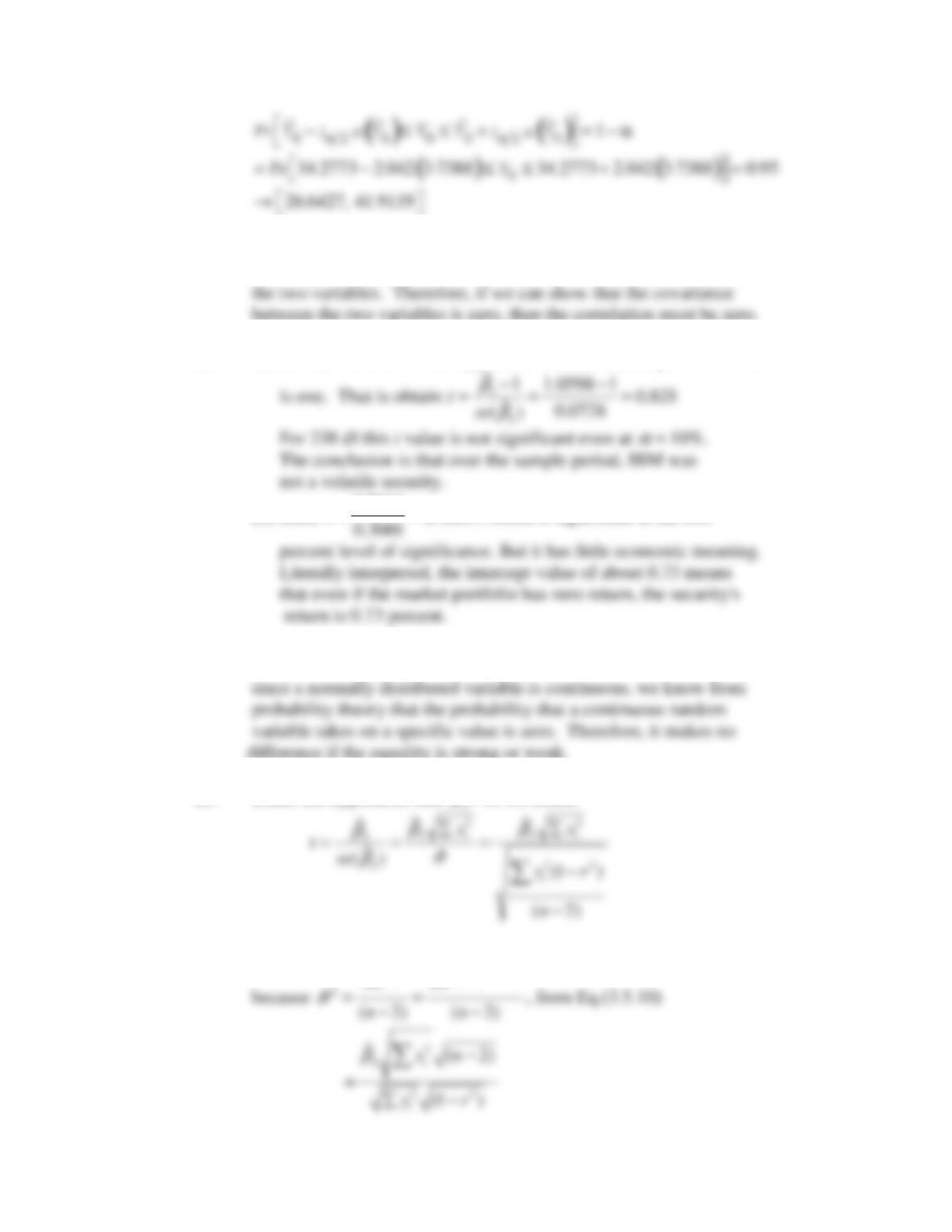
5.4 Verbally, the hypothesis states that there is no correlation between
5.5 (
a
) Use the
t
test to test the hypothesis that the true slope coefficient
(
b
) Since 0.7264
2.4205
t
= = , which is significant at the two
5.6 Under the normality assumption,
2
ˆ
β
is normally distributed. But
5.7 Under the hypothesis that
β
= 0, we obtain
2
2 2
ˆ
(1 )
i i
u y r
−
∑ ∑
Basic Econometrics, Gujarati and Porter
36
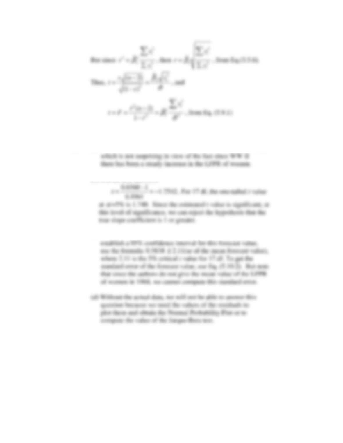
Empirical Exercises
5.8
(a) There is a positive association in the LFPR in 1972 and 1968,
(b) Use the one-tail t test.
(c) The mean LFPR is : 0.2033 + 0.6560 (0.58)
≈
0.5838. To
5.9
(a)
(b) Pay
i
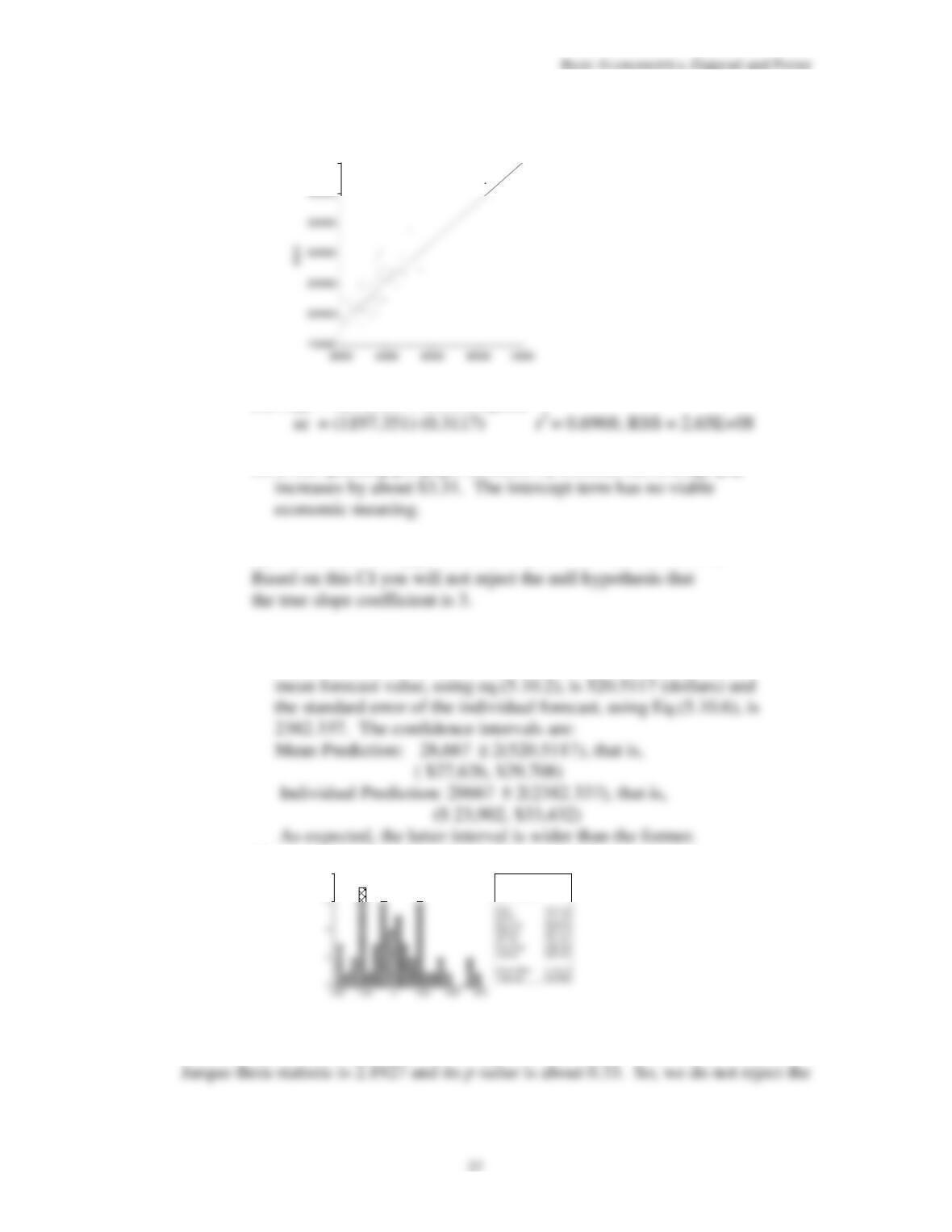
= 12129.37 + 3.3076 Spend
(c) If the spending per pupil increases by a dollar, the average pay
(d) The 95% CI for
2
β
is: 3.3076
±
2(0.3117) = (2.6842,3.931)
(e)The mean and individual forecast values are the same, namely,
12129.37 + 3.3076(5000)
≈
28,667. The standard error of the
(f)
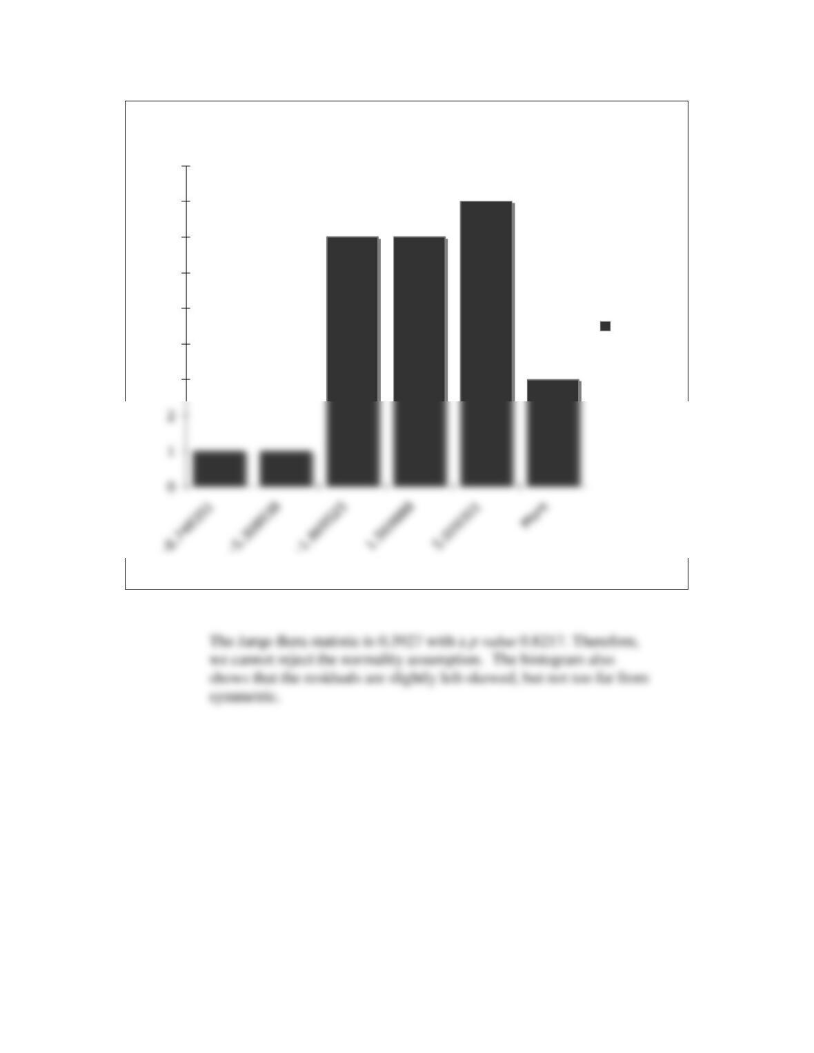
The histogram of the residuals can be approximated by a normal curve. The
45000
SPEND
8
Series: Residuals
Sample 1 51
Obs erv ations 51
38
5.10
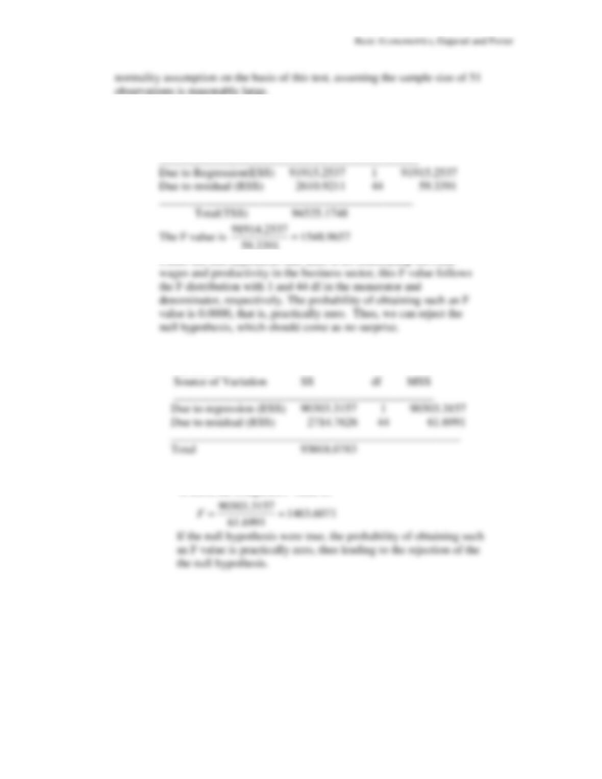
The ANOVA table for the business sector is as follows:
Source of Variation SS df MSS
Under the null hypothesis that there is no relationship between
(b) For the non-farm business sector, the ANOVA table is as
follows:
Under the null hypothesis that the true slope coefficient is
is zero, the computed F value is:
39
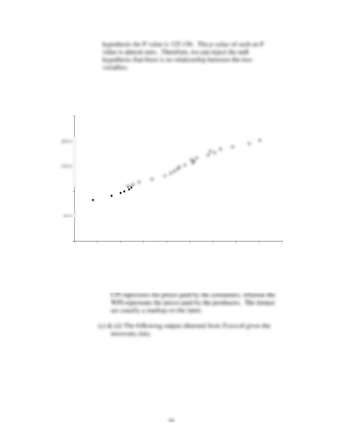
5.11
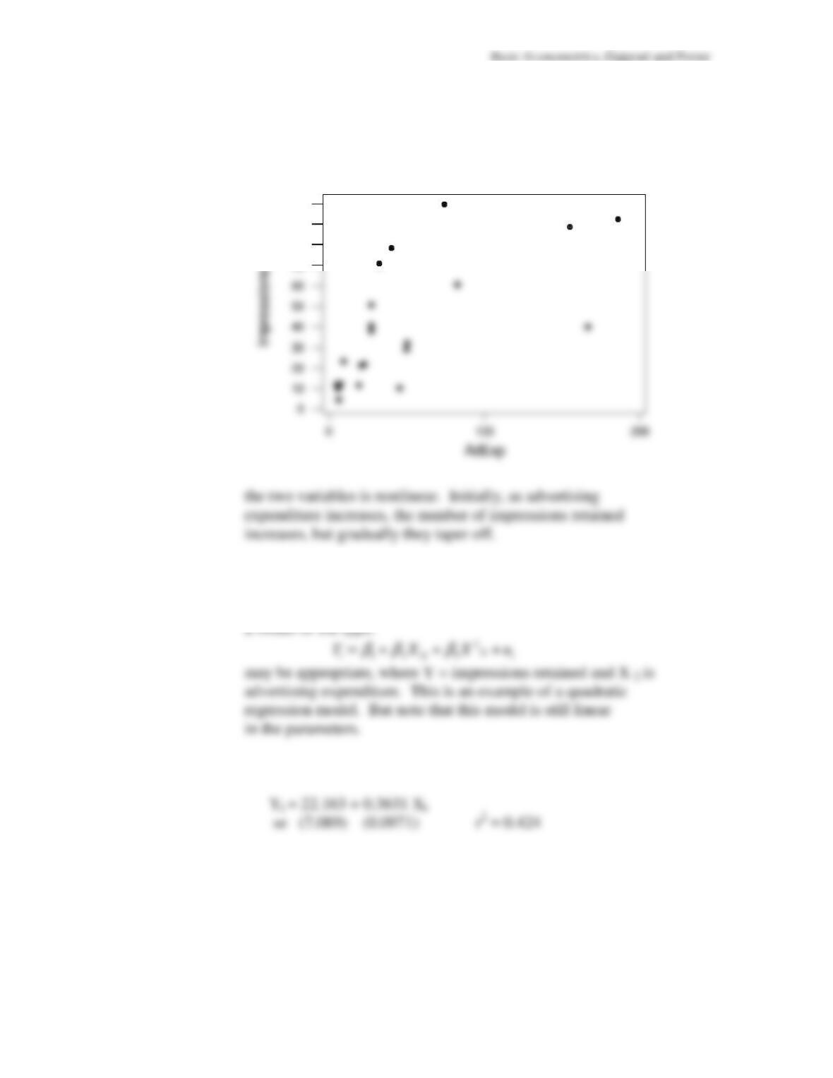
(a) The plot shown below indicates that the relationship between
(b) As a result, it would be inappropriate to fit a bivariate linear
regression model to the data. At present we do not have
the tools to fit an appropriate model. As we will show later,
(
c
) The results of blindly using a linear model are as follows:
100
90
80
70
5.12
(
a
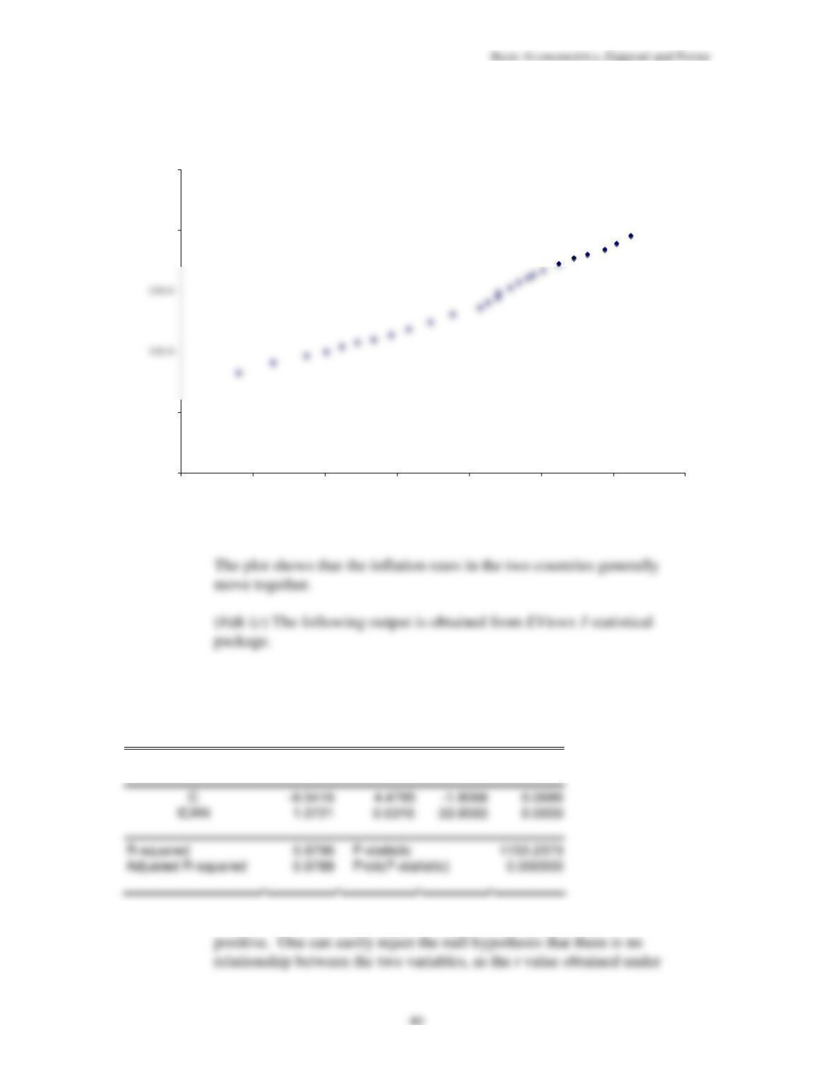
)
Sample: 1980 2005
Included observations: 26
Variable Coefficient
Std. Error
t-Statistic
Pr
ob.
As this output shows, the relationship between the two variables is
U.S. CPI vs Canada CPI
0.0
50.0
200.0
250.0
60.0 80.0 100.0 120.0 140.0 160.0 180.0 200.0
Candian CPI
41
5.13
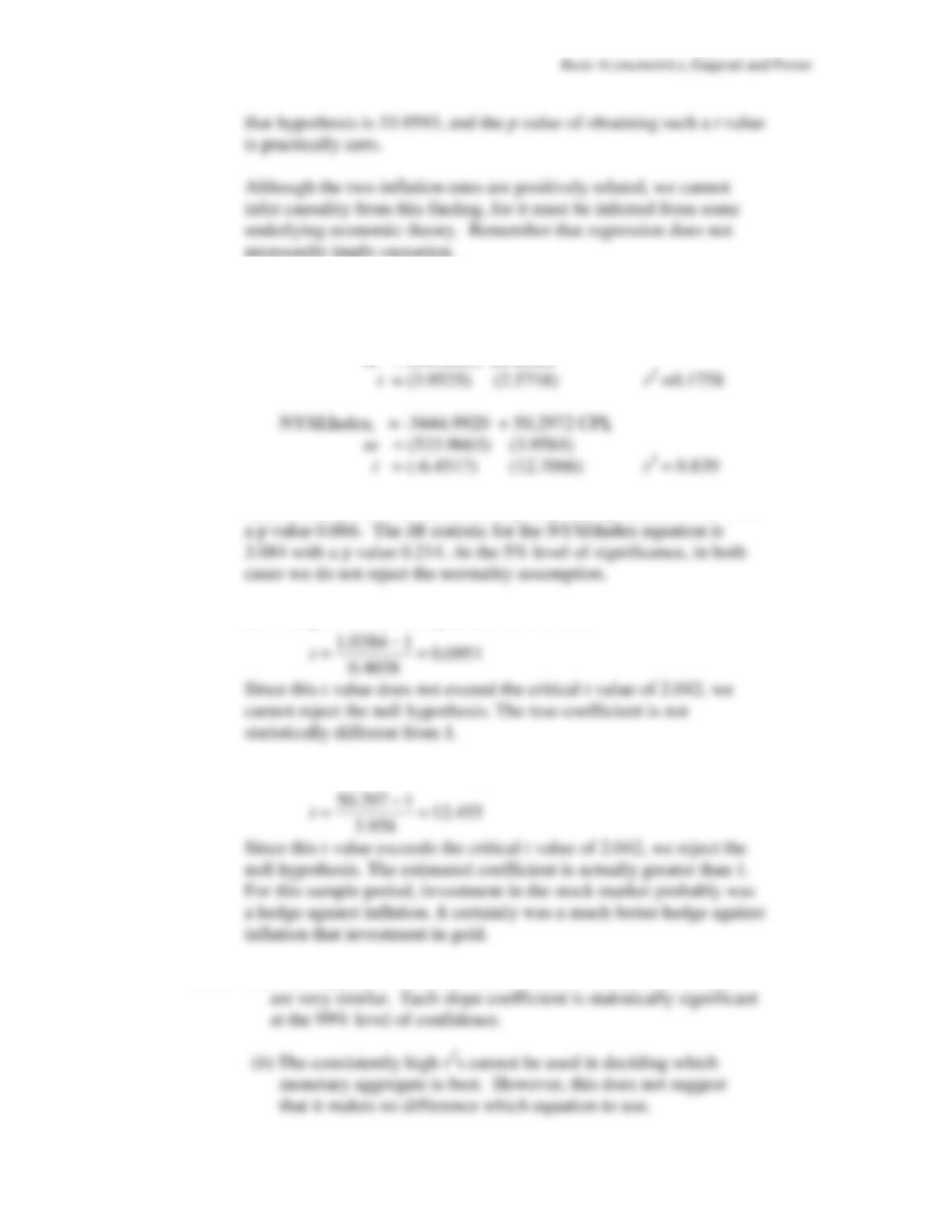
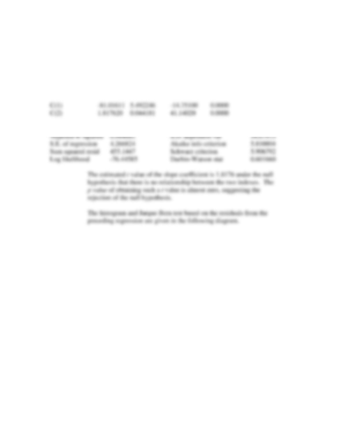
(a) The two regressions are as follows:
Goldprice
t
= 215.2856 + 1.0384 CPI
t
se
= (54.4685) (0.4038)
(b) The Jarqu-Bera statistic for the gold price equation is 5.439 with
(c) Using the usual t test procedure, we obtain:
(d) & (e) Using the usual t test procedure, we obtain:
5.14
(
a
) None appears to be better than the others. All statistical results
Basic Econometrics, Gujarati and Porter
42
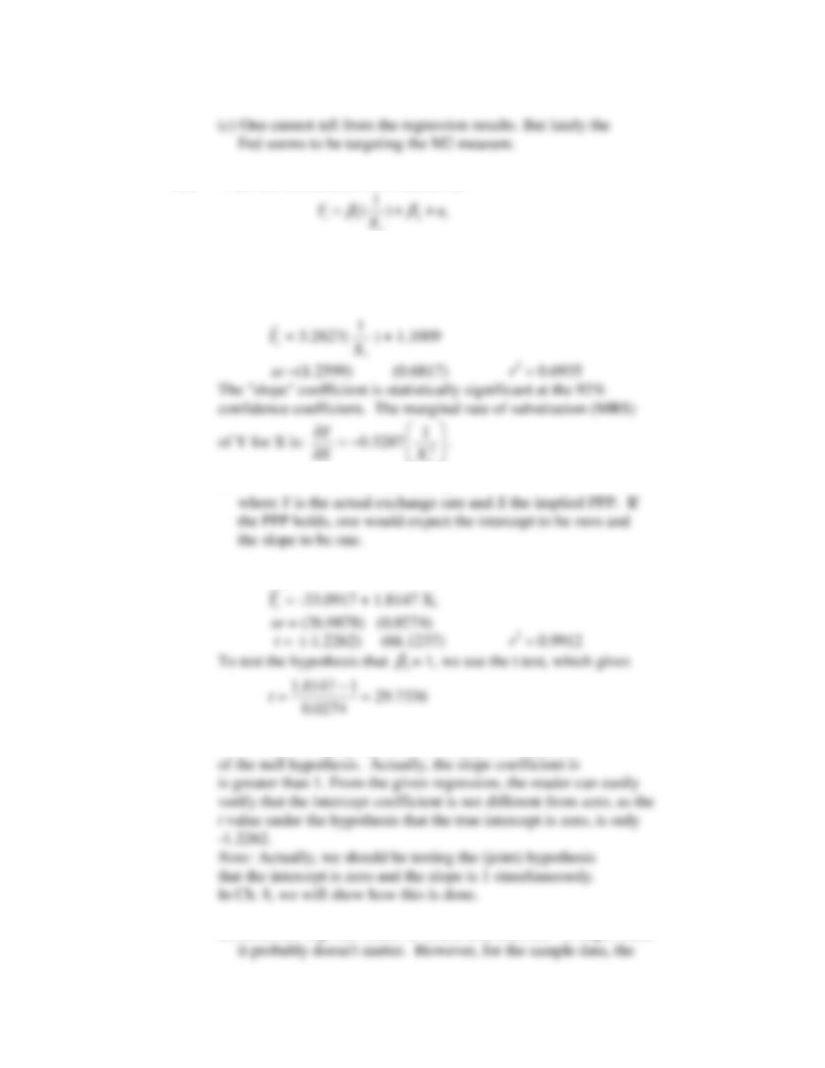
5.15
Write the indifference curve model as:
i
Note that now
1
β
becomes the slope parameter and
2
β
the intercept.
But this is still a linear regression model, as the parameters are
linear (more on this in Ch.6). The regression results are as follows:
i
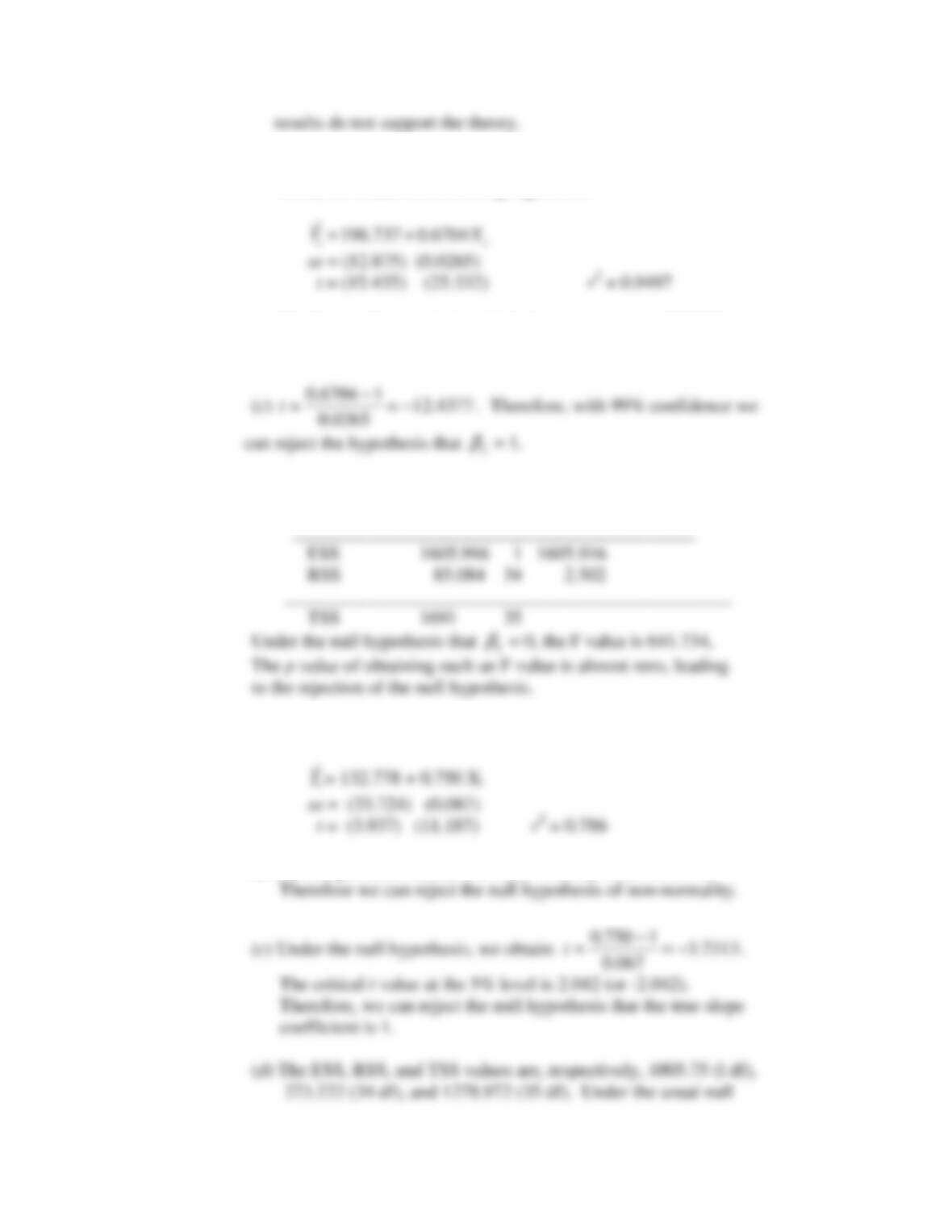
5.16
(
a
) Let the model be:
1 2 2
i i i
Y X u
β β
= + +
(
b
) The regression results are as follows:
This
t
value is highly significant, leading to the rejection
(
c
) Since the Big Max Index is “crude and hilarious” to begin with,
Basic Econometrics, Gujarati and Porter
43
5.17
(
a
) Letting Y represent the male math score and X the female math
score, we obtain the following regression:
(
b
) The Jarque-Bera statistic is 1.1641 with a
p value
of 0.5588.
Therefore, asymptotically we cannot reject the normality assumption.
(
d
) The ANOVA table is:
Source of Variation SS df MSS
5.18
(
a
) The regression results are as follows:
(
b
) The Jarque-Bera statistics is 1.122 with a
p value
of 0.571.
Basic Econometrics, Gujarati and Porter
5.19
(
a
)
CPI vs PPI (WPI)
0.0
100.0
250.0
80.0 90.0 100.0 110.0 120.0 130.0 140.0 150.0 160.0 170.0
PPI (WPI)
The scattergram as well is shown in the above figure.
(
b
) Treat CPI as the regressand and WPI as the regressor. The
Basic Econometrics, Gujarati and Porter
45
Dependent Variable: CPI
Method: Least Squares
Sample: 1980 2006
Included observations: 27
CPI=C(1)+C(2)*PPI
Coefficient Std. Error t-Statistic Prob.
R-squared 0.985444 Mean dependent var 142.3963
Basic Econometrics, Gujarati and Porter
46
Histogram
3
4
5
6
7
8
9
Bin
Frequency
47
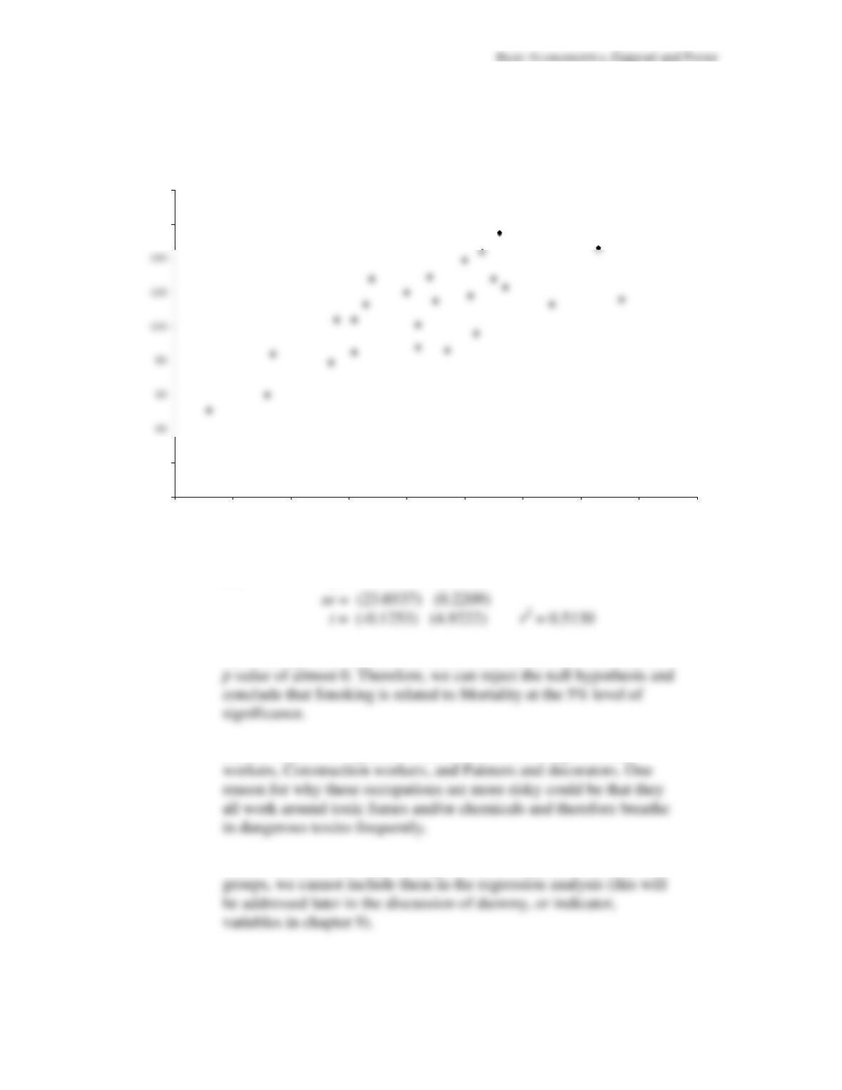
5.20
(a) There seems to be a general positive relationship between
Smoking and Mortality.
(b)
ˆ
i
Y
= -2.8853 + 1.0875 X
i
(c) The slope coefficient has a
t
statistic of 4.9222, which indicates a
(d) The riskiest occupations seem to be Furnace forge foundry
(e) Unless there is a way to categorize the occupations into fewer
Mortality vs Smoking
0
20
160
180
60 70 80 90 100 110 120 130 140 150
Smoking Index