Chapter 5
Hypothesis Tests and Model Selection
◼ Exercises
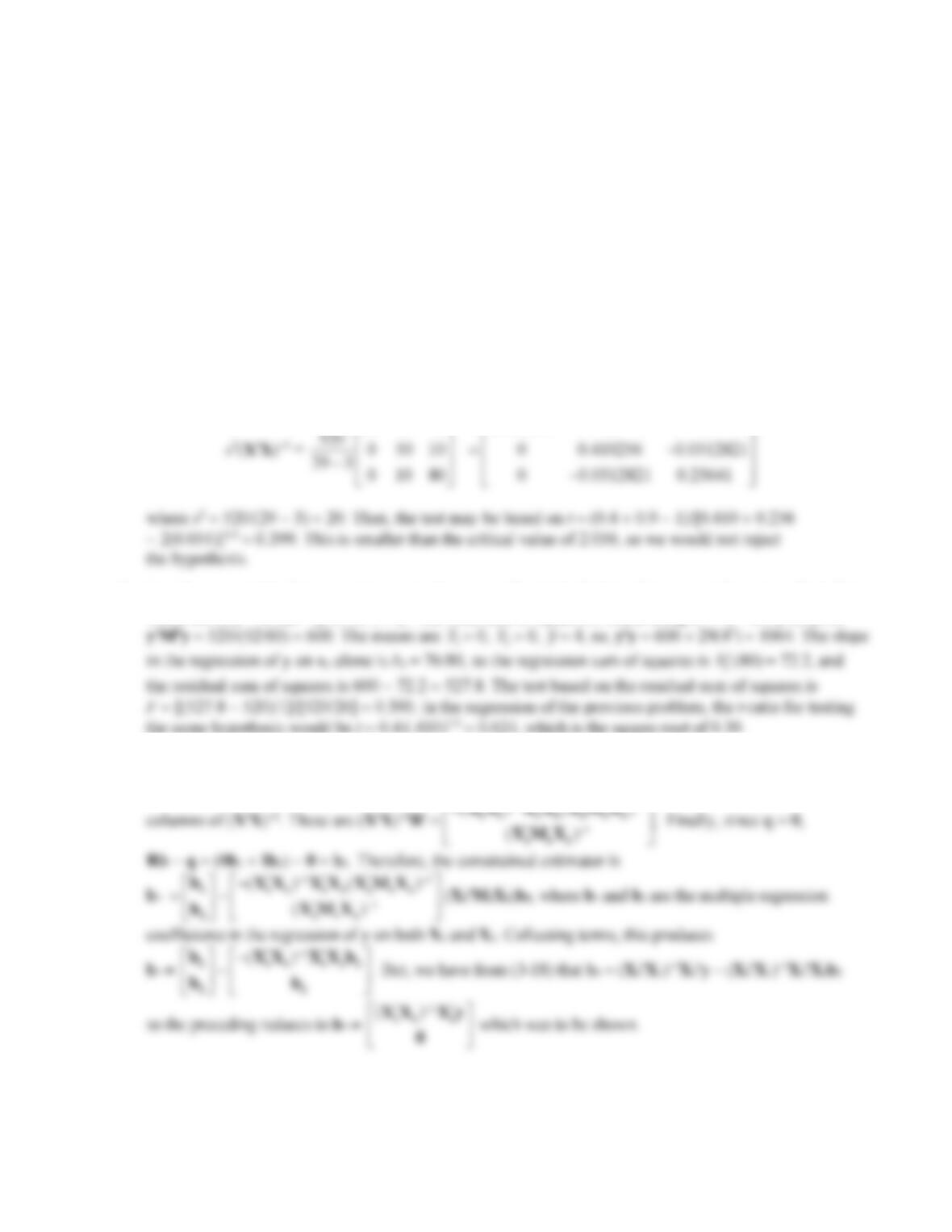
1. The estimated covariance matrix for the least squares estimator is
−
1
29 0 0 0.689655 0 0
2. In order to compute the regression, we must recover the original sums of squares and cross products for y.
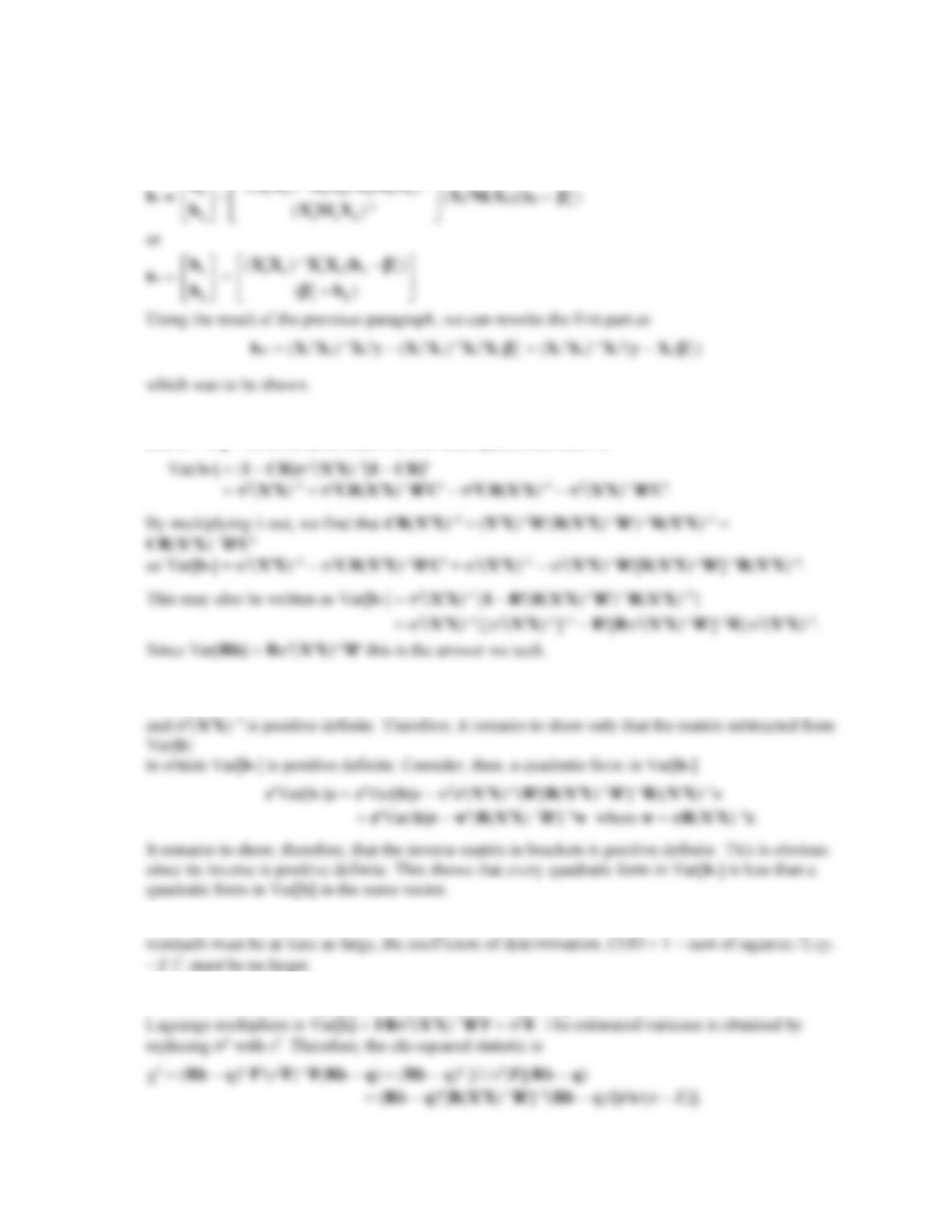
These are Xy = XXb = [116, 29, 76]. The total sum of squares is found using R2 = 1 − ee/yMy, so
the same hypothesis would be t = 0.4/(.410)1/2 = 0.624, which is the square root of 0.39.
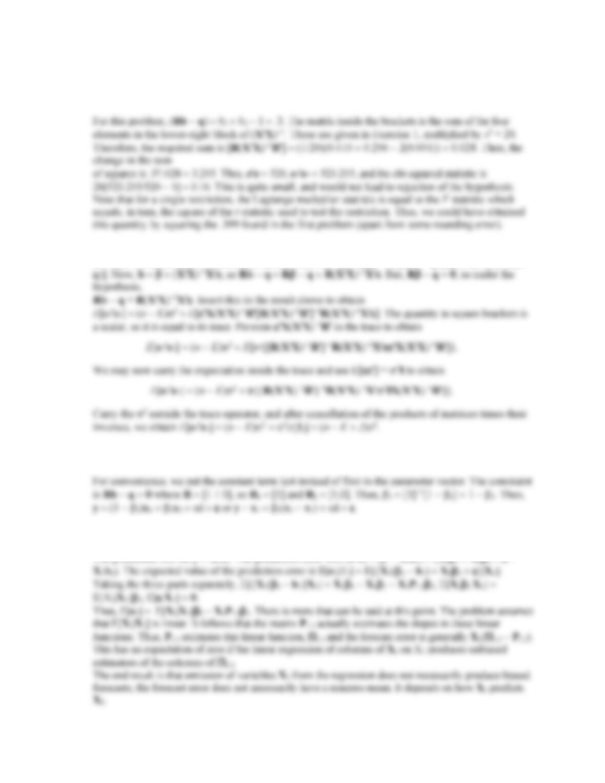
3. For the current problem, R = [0,I] where I is the last K2 columns. Therefore, R(XX)−1R is the lower
right K2 K2 block of (XX)−1. As we have seen before, this is (X2M1X2)−1. Also, (XX)−1R is the last K2
−−
11
If, instead, the restriction is 2 =
0
2
then the preceding is changed by replacing R − q = 0
with R −
0
2
= 0. Thus, Rb − q = b2 −
0
2.
Then, the constrained estimator is
−−
−
bX X X X X M X
11
( ) ( )
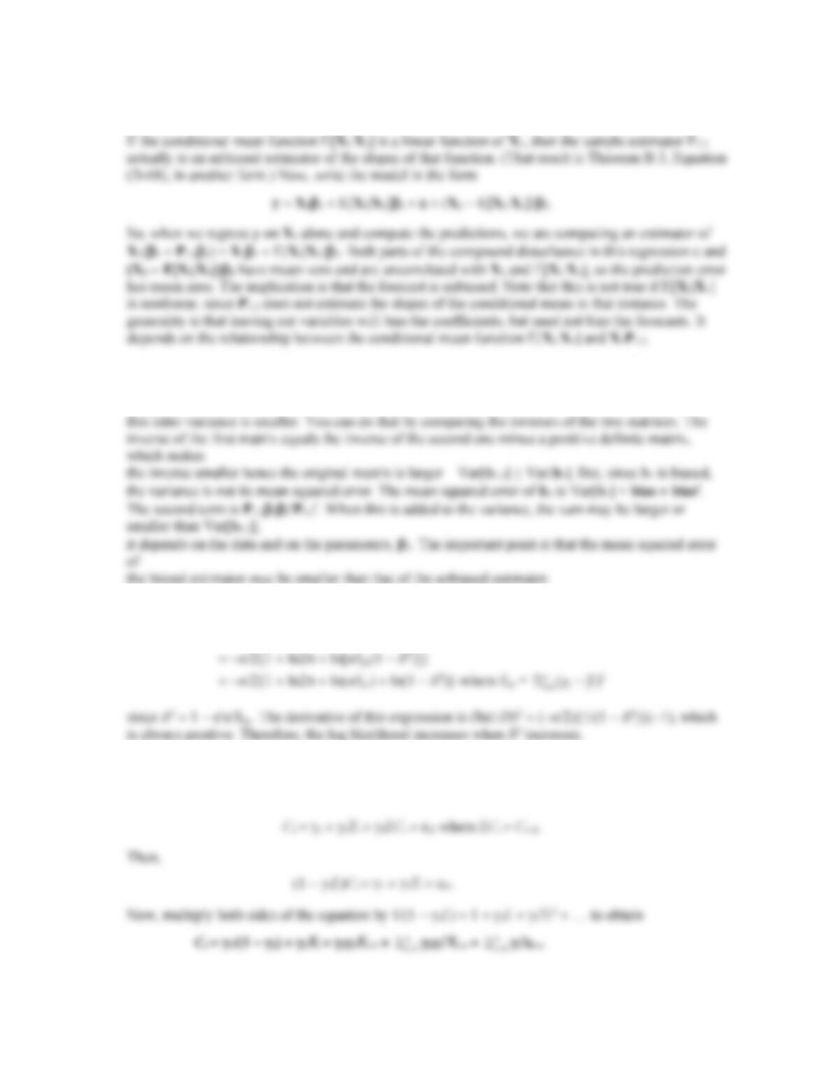
4. By factoring the result in (5-23), we obtain b* = [I − CR]b + w where C = (XX)−1R[R(XX)−1R]−1
and w = Cq. The covariance matrix of the least squares estimator is
5. The variance of the restricted least squares estimator is given in the second equation in the previous
exercise. We know that this matrix is positive definite, since it is derived in the form B2(XX)−1B,
6. The result follows immediately from the result which precedes (5-28). Since the sum of squared
7. For convenience, let F = [R(XX)−1R]−1. Then, = F(Rb − q) and the variance of the vector of

8. We use (5-28) to find the new sum of squares. The change in the sum of squares is
e*e* − ee = (Rb − q) [R(XX)−1R]−1(Rb − q).
9. First, use (5-28) to write e*e* = ee + (Rb − q)[R(XX)−1R]−1(Rb − q). Now, the result that E[ee] =
(n − K)2 obtained in (4-17) must hold here, so E[e*e*] = (n − K)2 + E[(Rb − q)[R(XX)−1R]−1(Rb −
10. Show that in the multiple regression of y on a constant, x1, and x2, while imposing the restriction
1 + 2 = 1 leads to the regression of y − x1 on a constant and x2 − x1.
11. If the regression model is y = X11 + X22 + , and y is regressed on X1 alone, then E[b1] = 1 +
P1.22.
The prediction will be y = X1b1. The prediction error will be e1 = (y − X1b1) = (X11 + X22 + −
The result cited is E[b1] = 1 + P1.22 where P1.2 = (X1X1)−1X1X2, so the coefficient estimator is
biased.
12. The “long” estimator, b1.2 is unbiased, so its mean squared error equals its variance, 2(X1M2X1)−1
The short estimator, b1 is biased; E[b1] = 1 + P1.22. Its variance is 2(X1X1)−1. It is easy to show
that
13. The log likelihood function at the maximum is
lnL = −n/2[1 + ln2 + ln(ee/n)]
14. An inconvenient way to obtain the result is by repeated substitution of Ct–1, then Ct–2 , and so on. It is
much easier and faster to introduce the lag operator used in Chapter 20. Thus, the alternative model
is
Applications
?=======================================================================
? Application 5.1 Wage Equation
?=======================================================================
Read;File=…; nvar=5;nobs=17919$
? This creates the group count variable.
Regress ; Lhs = one ; Rhs = one ; Str = ID ; Panel $
?=======================================================================
? a. Long regression
?=======================================================================
regress ; lhs= lwage ; rhs = x1,x2 $
+—————————————————-+
| Ordinary least squares regression |
| LHS=LWAGE Mean = 2.296821 |
| Standard deviation = .5282364 |
+—————————————————-+
+——–+————–+—————-+——–+——–+———-+
|Variable| Coefficient | Standard Error |b/St.Er.|P[|Z|>z]| Mean of X|
+——–+————–+—————-+——–+——–+———-+
Constant| .98965433 .03389449 29.198 .0000
?=======================================================================
? b. F test
?=======================================================================
Calc ; list ; fstat = Rsqrd/(kreg-1)/((1-rsqrd)/(n-kreg)) $
+————————————+
FSTAT = 14.025040
+—————————————————-+
| Ordinary least squares regression |
| LHS=LWAGE Mean = 2.296821 |
| Standard deviation = .5282364 |
+—————————————————-+
+——–+————–+—————-+——–+——–+———-+
|Variable| Coefficient | Standard Error |b/St.Er.|P[|Z|>z]| Mean of X|
+——–+————–+—————-+——–+——–+———-+
Constant| 1.02722913 .03004146 34.194 .0000
?=======================================================================
? c. F test for hypothesis that coefficients on X2 are zero
?=======================================================================
Calc ; list ; fstat = (r1-rsqrd)/(col(x2))/((1-r1)/(df1)) $
?=======================================================================
? d. Wald test for hypothesis that coefficients on X2 are zero
?=======================================================================
1| 56.10016
Note Wald = 4*F, as expected.
?=======================================================================
? Application 5.2 Translog Cost Function
?=======================================================================
? First prepare the data
?
Create ; lpk=log(pk);lpl=log(pl);lpf=log(pf)$
?=======================================================================
? a. Beta is a,b,dk,dl,df,pkk,pll,pff,pkl,pkf,plf,c,tqk,tql,tqf
?=======================================================================
Restrictions are
?=======================================================================
? b. Testing the theory
?=======================================================================
Namelist ; X1=one,lq,lpk,lpl,lpf,lpk2,lpl2,lpf2,lpkl,lpkf,lplf,lq2,lqk,lq…
Namelist ; X0=one,lq,lpkf,lplf,lpkpf2,lplpf2,lplfpkf,lq2,lqlpkf,lqlplf$
Regress ; lhs = lc ; rhs=x0 $
+—————————————————-+
| Ordinary least squares regression |
| LHS=LC Mean = 3.071619 |
| Standard deviation = 1.542734 |
+—————————————————-+
+——–+————–+—————-+——–+——–+———-+
|Variable| Coefficient | Standard Error |t-ratio |P[|T|>t]| Mean of X|
+——–+————–+—————-+——–+——–+———-+
Constant| -1.13340208 1.04296294 -1.087 .2789
LQ | .02244828 .12717485 .177 .8601 8.26548908
LPKF | -.02309567 .14153592 -.163 .8706 14.4192992
Calc ; ee0 = sumsqdev $
+—————————————————-+
| Ordinary least squares regression |
| LHS=LCPF Mean = -.3195570 |
| Standard deviation = 1.542364 |
+—————————————————-+
+——–+————–+—————-+——–+——–+———-+
|Variable| Coefficient | Standard Error |t-ratio |P[|T|>t]| Mean of X|
+——–+————–+—————-+——–+——–+———-+
Constant| -76.2592615 38.2800363 -1.992 .0483
LPL | 14.7182926 7.08482345 2.077 .0395 8.97279814
LPF | -1.89473291 2.84231282 -.667 .5061 3.39117564
LPK2 | -.32741427 .44070869 -.743 .4587 9.05539681
LPL2 | -1.53852735 .69240298 -2.222 .0279 40.2700121
Calc ; ee1 = sumsqdev $
FSTAT = 1.973714
+————————————+
Result = 2.277490
The F statistic is small; the theory is not rejected.
?=======================================================================
? c. Testing homotheticity
?=======================================================================
+—————————————————-+
| Ordinary least squares regression |
| LHS=LCPF Mean = -.3195570 |
| Standard deviation = 1.542364 |
+—————————————————-+
+——–+————–+—————-+——–+——–+———-+
|Variable| Coefficient | Standard Error |t-ratio |P[|T|>t]| Mean of X|
+——–+————–+—————-+——–+——–+———-+
Constant| -2.78239562 1.04292476 -2.668 .0085
LQ | .01362521 .12717020 .107 .9148 8.26548908
LPKF | -.06044098 .14153074 -.427 .6700 14.4192992
+—————————————————-+
| Linearly restricted regression |
| Ordinary least squares regression |
| LHS=LCPF Mean = -.3195570 |
| Standard deviation = 1.542364 |
| Model test F[ 7, 150] (prob) =2741.96 (.0000) |
+——–+————–+—————-+——–+——–+———-+
|Variable| Coefficient | Standard Error |t-ratio |P[|T|>t]| Mean of X|
+——–+————–+—————-+——–+——–+———-+
Constant| -6.20547247 .37175165 -16.693 .0000
LQ | .40111764 .03208201 12.503 .0000 8.26548908
LPKF | -.05918207 .14502101 -.408 .6838 14.4192992
?=======================================================================
? d. Testing generalized Cobb-Douglas against full translog
?=======================================================================
Regress ; lhs = lcpf ; rhs = x0 ;cls:b(5)=0,b(6)=0,b(7)=0,b(9)=0,b(10)=0$
+—————————————————-+
| Linearly restricted regression |
| Ordinary least squares regression |
| LHS=LCPF Mean = -.3195570 |
| Standard deviation = 1.542364 |
+——–+————–+—————-+——–+——–+———-+
|Variable| Coefficient | Standard Error |t-ratio |P[|T|>t]| Mean of X|
+——–+————–+—————-+——–+——–+———-+
Constant| -5.07718678 .18072495 -28.093 .0000
LQ | .41724916 .03285950 12.698 .0000 8.26548908
LQLPLF | -.693889D-17 .223074D-09 .000 1.0000 251.570118
+————————————+
| Listed Calculator Results |
+————————————+
?=======================================================================
? e. Testing Cobb-Douglas against full translog
1
+————–
+————————————+
| Listed Calculator Results |
+————————————+
The F statistic of 28.871 is larger than the critical value of 2.16. The hypothesis
is rejected.
?=======================================================================
? f. Testing generalized Cobb-Douglas against homothetic translog
+—————————————————-+
| Linearly restricted regression |
| Ordinary least squares regression |
| LHS=LCPF Mean = -.3195570 |
| Standard deviation = 1.542364 |
| WTS=none Number of observs. = 158 |
+—————————————————-+
+——–+————–+—————-+——–+——–+———-+
|Variable| Coefficient | Standard Error |t-ratio |P[|T|>t]| Mean of X|
+——–+————–+—————-+——–+——–+———-+
Constant| -5.07718678 .18072495 -28.093 .0000
LQ | .41724916 .03285950 12.698 .0000 8.26548908
Calc ; list ; ftb(.95,3,150) $
+————————————+
?
?=======================================================================
? g. We have not rejected the theory, but we have rejected all the
? functional forms
? except the nonhomothetic translog. Just like Christensen and Greene.
?=======================================================================
?=======================================================================
? Application 5.3 Nonlinear Restrictions
?=======================================================================
sample;1-52$
name;x=one,logpg,logi,logpnc,logpuc,logppt,t,logpd,logpn,logps$
?=======================================================================
? a. Simple hypothesis test
?=======================================================================
Regr;lhs=logg;rhs=x$
+—————————————————-+
| Ordinary least squares regression |
| LHS=LOGG Mean = 1.570475 |
+—————————————————-+
+——–+————–+—————-+——–+——–+———-+
|Variable| Coefficient | Standard Error |t-ratio |P[|T|>t]| Mean of X|
+——–+————–+—————-+——–+——–+———-+
Constant| -7.28719016 2.52056245 -2.891 .0061
LOGPG | .06051812 .05401018 1.120 .2689 3.72930296
LOGI | .99299135 .25037574 3.966 .0003 9.67214751
+—————————————————-+
| Ordinary least squares regression |
| LHS=LOGG Mean = 1.570475 |
| Standard deviation = .2388115 |
+—————————————————-+
+——–+————–+—————-+——–+——–+———-+
|Variable| Coefficient | Standard Error |t-ratio |P[|T|>t]| Mean of X|
+——–+————–+—————-+——–+——–+———-+
Constant| -13.1396625 2.09171186 -6.282 .0000
LOGPG | -.05373342 .04251099 -1.264 .2127 3.72930296
Calc;r0=rsqrd$
Calc;list;f=((r1-r0)/2)/((1-r1)/(n-10))$
?=======================================================================
? b. Nonlinear restriction
?=======================================================================
Since the restricted model is nonlinear, it would be quite cumbersome to estimate and examine the loss in
fit. We can test the restriction using the unrestricted model. For this problem,
f = [nc − uc, ncs − ptd]
The matrix of derivatives, using the order given above and “ to represent the entire parameter vector, is
(a).
Thus, f = [− 0.17399, .10091]. The covariance matrix to use for the tests is Gs2(XX)−1G.
Neither is large, so neither hypothesis would be rejected. (Given the earlier result, this was to be
expected.)
?=======================================================================
? c. Computations for nonlinear restriction
?=======================================================================
sample;1-52$
name;x=one,logpg,logi,logpnc,logpuc,logppt,t,logpd,logpn,logps$
Regr;lhs=logg;rhs=x$
+—————————————————-+
| Ordinary least squares regression |
| LHS=LOGG Mean = 1.570475 |
| Model test F[ 6, 45] (prob) = 207.55 (.0000) |
+—————————————————-+
+——–+————–+—————-+——–+——–+———-+
|Variable| Coefficient | Standard Error |t-ratio |P[|T|>t]| Mean of X|
+——–+————–+—————-+——–+——–+———-+
Constant| -13.1396625 2.09171186 -6.282 .0000
LOGPG | -.05373342 .04251099 -1.264 .2127 3.72930296
+—————————————————-+
| Ordinary least squares regression |
| LHS=LOGG Mean = 1.570475 |
| Standard deviation = .2388115 |
+——–+————–+—————-+——–+——–+———-+
|Variable| Coefficient | Standard Error |t-ratio |P[|T|>t]| Mean of X|
+——–+————–+—————-+——–+——–+———-+
Constant| -13.1396625 2.09171186 -6.282 .0000
LOGPG | -.05373342 .04251099 -1.264 .2127 3.72930296
+————————————+
Result = 2.827049
REGR;Lhs=logg;rhs=x$
1
+————–
2| .10091

Calc;list;z1=f(1)/sqr(vf(1,1))$
The J test in Example 5.7 is carried out using over 50 years of data. It is optimistic to hope that the
?====================================
? Example Application 5.4
?====================================
Dates ; 1950.1 $
| Ordinary least squares regression |
| Model was estimated May 12, 2007 at 08:56:19AM |
| LHS=CT Mean = 3008.995 |
| Model test F[ 3, 199] (prob) =******* (.0000) |
| Diagnostic Log likelihood = -886.1351 |
+—————————————————-+
+——–+————–+—————-+——–+——–+———-+
|Variable| Coefficient | Standard Error |t-ratio |P[|T|>t]| Mean of X|
+——–+————–+—————-+——–+——–+———-+
Constant| -.60444607 3.43245774 -.176 .8604
+—————————————————-+
| Ordinary least squares regression |
| Model was estimated May 12, 2007 at 08:56:19AM |
| LHS=CT Mean = 3008.995 |
| Standard error of e = 19.22496 |
| Fit R-squared = .9998285 |
+—————————————————-+
+——–+————–+—————-+——–+——–+———-+
|Variable| Coefficient | Standard Error |t-ratio |P[|T|>t]| Mean of X|
+——–+————–+—————-+——–+——–+———-+
Constant| -865.712368 120.569071 -7.180 .0000
? Application 7.1. We use only the 1980 data, so we
? start in quarter 2 of 1980 even though data are
? available for the last quarter of 1979.
+—————————————————-+
| Ordinary least squares regression |
| Model was estimated May 12, 2007 at 08:58:19AM |
| LHS=CT Mean = 4503.230 |
| Standard deviation = 879.3593 |
| WTS=none Number of observs. = 83 |
+—————————————————-+
+——–+————–+—————-+——–+——–+———-+
|Variable| Coefficient | Standard Error |t-ratio |P[|T|>t]| Mean of X|
+——–+————–+—————-+——–+——–+———-+
Constant| 39.6958824 37.1402619 1.069 .2884
Regress; Lhs = Ct ; Rhs = one,Yt,Ct1,CY $
+—————————————————-+
| Ordinary least squares regression |
| Model was estimated May 12, 2007 at 08:58:19AM |
| LHS=CT Mean = 4503.230 |
+—————————————————-+
+——–+————–+—————-+——–+——–+———-+
|Variable| Coefficient | Standard Error |t-ratio |P[|T|>t]| Mean of X|
+——–+————–+—————-+——–+——–+———-+
?
? The results are essentially the same. This suggests
? that neither model is right.