
CHAPTER 5
TEACHING NOTES
Chapter 5 is short, but it is conceptually more difficult than the earlier chapters, primarily
because it requires some knowledge of asymptotic properties of estimators. In class, I give a
brief, heuristic description of consistency and asymptotic normality before stating the
An explicit illustration of what happens to standard errors as the sample size grows emphasizes
the importance of having a larger sample. I do not usually cover the LM statistic in a first-
semester course, and I only briefly mention the asymptotic efficiency result. Without full use of
matrix algebra combined with limit theorems for vectors and matrices, it is difficult to prove
asymptotic efficiency of OLS.
49
SOLUTIONS TO PROBLEMS
5.1 Write y =
0
+
1
x1 + u, and take the expected value: E(y) =
0
+
1
E(x1) + E(u), or µy =
PLIM.2 from Appendix C.
5.2 A higher tolerance of risk means more willingness to invest in the stock market, so
2
> 0.
5.4 Write y =
0
+
1
x + u, and take the expected value: E(y) =
0
+
1
E(x) + E(u), or µy =
1
1
SOLUTIONS TO COMPUTER EXERCISES
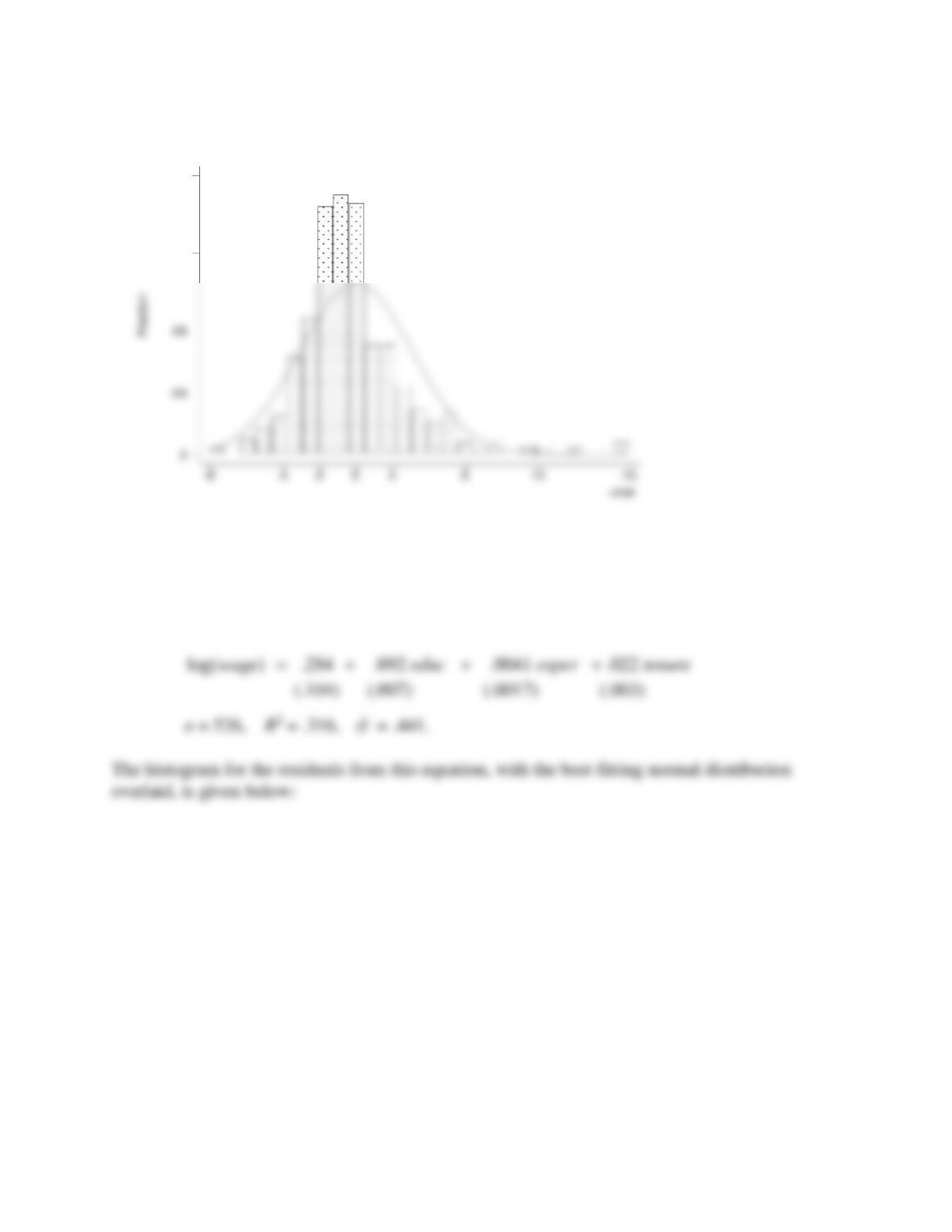
C5.1 (i) The estimated equation is
0
50
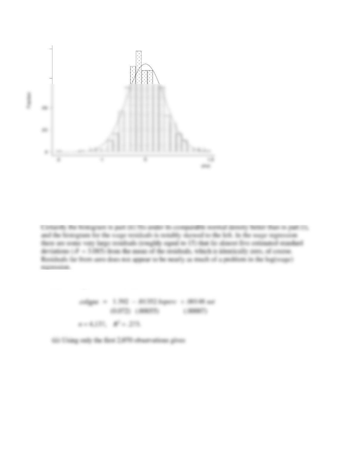
(ii) With log(wage) as the dependent variable the estimated equation is
.13
.18
51
(iii) The residuals from the log(wage) regression appear to be more normally distributed.
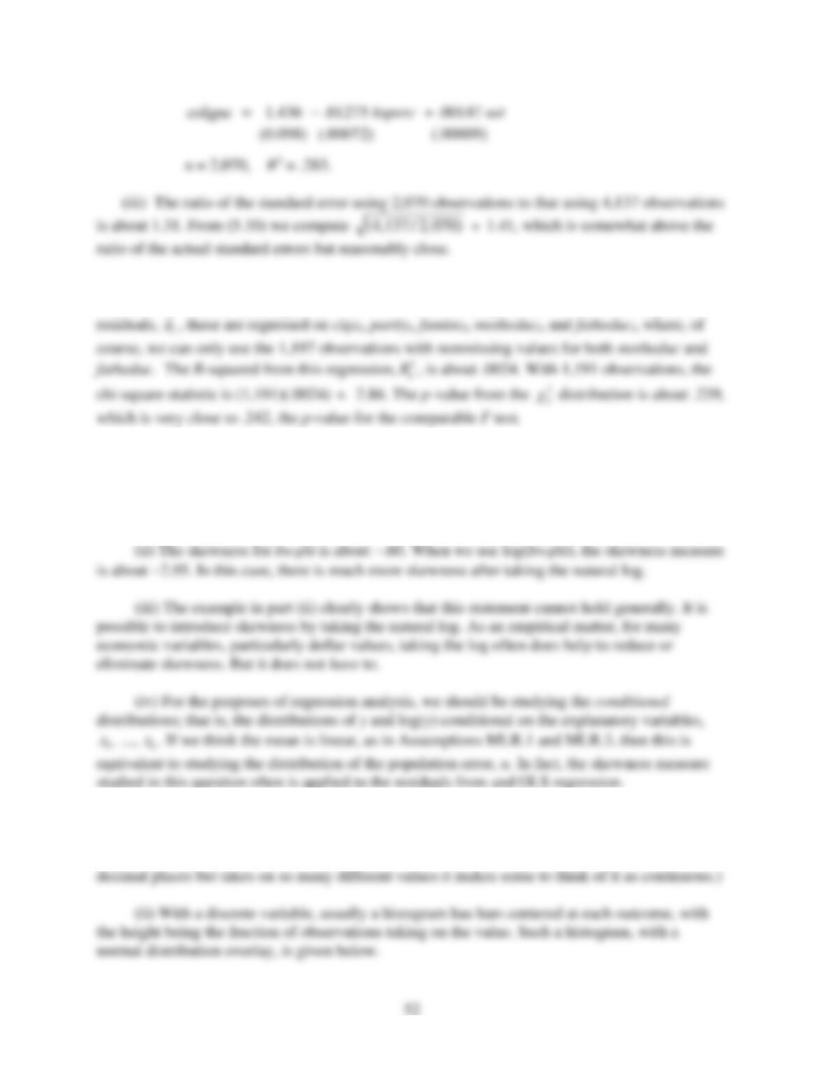
C5.2 (i) The regression with all 4,137 observations is
.1
.14
C5.3 We first run the regression colgpa on cigs, parity, and faminc using only the 1,191
observations with nonmissing observations on motheduc and fatheduc. After obtaining these
C5.4 (i) The measure of skewness for inc is about 1.86. When we use log(inc), the skewness
measure is about .360. Therefore, there is much less skewness in log of income, which means inc
is less likely to be normally distributed. (In fact, the skewness in income distributions is a well-
documented fact across many countries and time periods.)
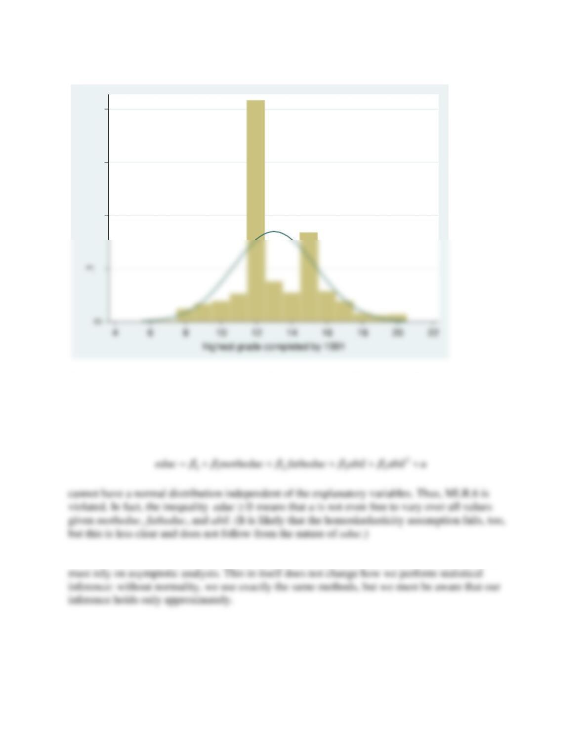
C5.5 (i) The variable educ takes on all integer values from 6 to 20, inclusive. So it takes on 15
distinct values. It is not a continuous random variable, nor does it make sense to think of it as
approximately continuous. (Contrast a variable such as hourly wage, which is rounded to two
53
Even discounting the discreteness, the best fitting normal distribution (matching the sample
mean and variance) fits poorly. The focal point at educ = 12 clearly violates the notion of a
smooth bell-shaped density.
(iv) Given the findings in part (iii), the error term in the equation
(v) The violation of MLR.6 means that we cannot perform exact statistical inference; we
density