1
CHAPTER 4
Uncertainty
A. Summary
Chapter 4 provides a foundation for students to help understand the important
role that uncertainty and information theory has come to play in microeco-
nomics. This material appears early in the text for two reasons: first, so that it
can be used occasionally in subsequent chapters (including for example the
chapter on game theory, where uncertainty comes up in the discussion of
B. Lecture and Discussion Suggestions
With the huge volume of material that needs to be covered in an intermediate
microeconomics course, the instructor needs to pare down what is covered to
fit into a sensible one-semester course. There is a great temptation to omit
Courses in business schools may want to include coverage of Section
4.4 on financial applications.
The appendix model essentially goes through all the same material a
second time using a different model. Many instructors will choose to omit
Chapter 4: Uncertainty
2
two-state model, is to focus their lectures entirely around the appendix and
have the students read the earlier material as background.
The concepts in this chapter are perhaps a bit more difficult than in some
other chapters. More repetition of material in the book may be required in
C. Glossary Entries in the Chapter
• Diversification
• Expected value
D. Notes on Review Questions
Review Question 3. Some background might help the instructor if stu-
dents have questions with this one. We generated the example assuming that
gamble 1 has a 50-50 chance of paying off 0 or 100. Gamble 2 has a ¾
chance of paying off 0 and ¼ chance of paying off 300. The assumed utility
function is
()U I I=
.
SOLUTIONS TO CHAPTER 4 PROBLEMS
4.1 a. Given that these are actual gambles offered in Las Vegas, you shouldn’t be
surprised to learn that they are unfair in the casino’s favor. To verify this
claim, we can compute the expected payoff from gamble 1,
Chapter 4: Uncertainty
3
They are both negative, not zero as required of fair gambles.
b. To figure out which gamble Wen would take, compute the expected utility
from gamble 1,
The first is higher, so Wen would choose gamble 1.
c. The expected utility from not taking either gamble is the same as the utility
from current income ($10,000) with certainty:
10,000 100=
. This is higher
4.2 a. E(1) = .50(100) + .50(–100) = 0
E(2) = .75(100) + .25(–300) = 0
E(3) = .90(100) + .10(–900) = 0
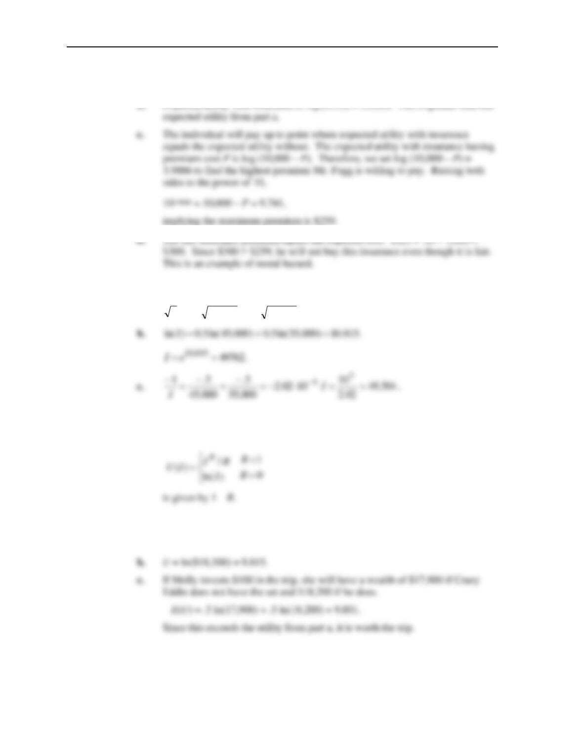
b. Assume current income is $1,000. Then utility of income graph is:
Chapter 4: Uncertainty
4
4.3 a. Expected utility without insurance is .75 log(10,000) + .25 log(9,000) =
3.9886.
4.4 a.
875,4965.446000,555.0000,455.0 ==+= II
.
The functions exhibit increasingly greater risk aversion. This is an illustration
of the general principle that the degree of (relative) risk aversion for the utility
function
4.5 a. U = ln($18,000) = 9.798.
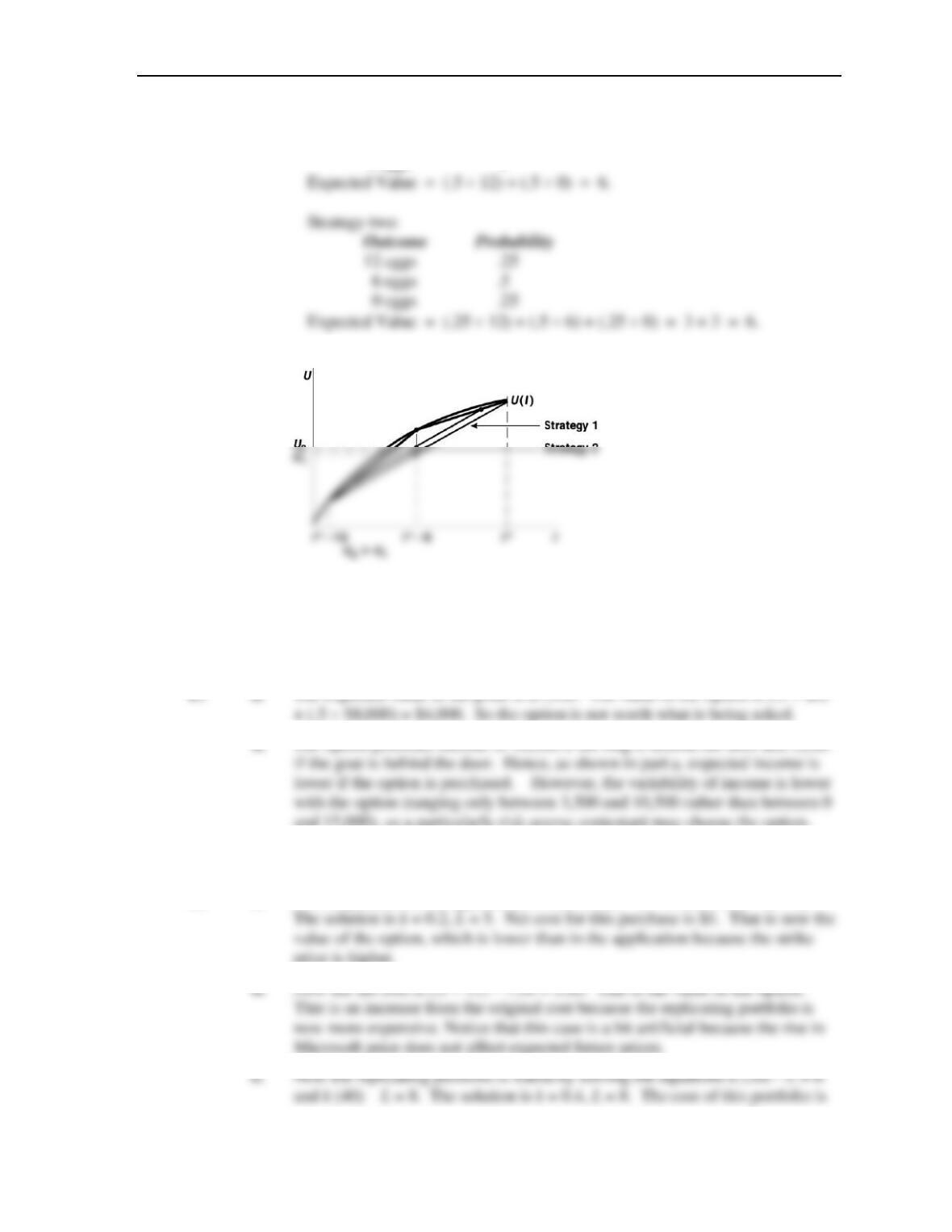
4.6 a. Strategy one:
Chapter 4: Uncertainty
5
Outcome Probability
12 eggs .5
0 eggs .5
b.
c. Gains from diversification are offset by costs of extra trips, so there may be an
optimal number of such trips.
4.7 a. The expected value of the prize is $7,500. The value of the option is (.5 $0)
b. The option promises income of 10,500 if the ring is behind the door and 3,500
and 15,000), so a particularly risk-averse contestant may choose the option.
4.8 a. Now Equations (1) in Application 4.4 are k (25) – L = 0 and k (35) – L = 2.
price is higher.
Chapter 4: Uncertainty
6
$4. This is an increase from the value in the application because of the in-
creased volatility in the share price.
d. Interest payments can be treated as creating a difference between the amount
borrowed and the amount repaid. If, for example, the interest rate were 5 per-
4.9 a. With the first utility function, we have
000,985.0000,1165.0 +=I
,
b. With this extreme utility function,
101010 )000,98(5.0)000,116(5.0 −−− +=I
4.10 a. Leah’s initial situation without insurance is shown as point A in the graph.
Full, fair insurance moves her to point B. Full insurance at unfair terms moves
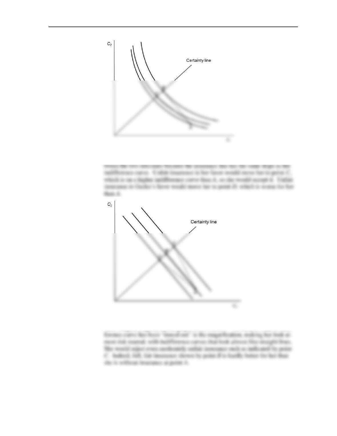
Chapter 4: Uncertainty
7
b. If Leah is risk neutral, her indifference curves are straight lines. Full, fair in-
surance moves her from uninsured point A to point B. She is indifferent be-
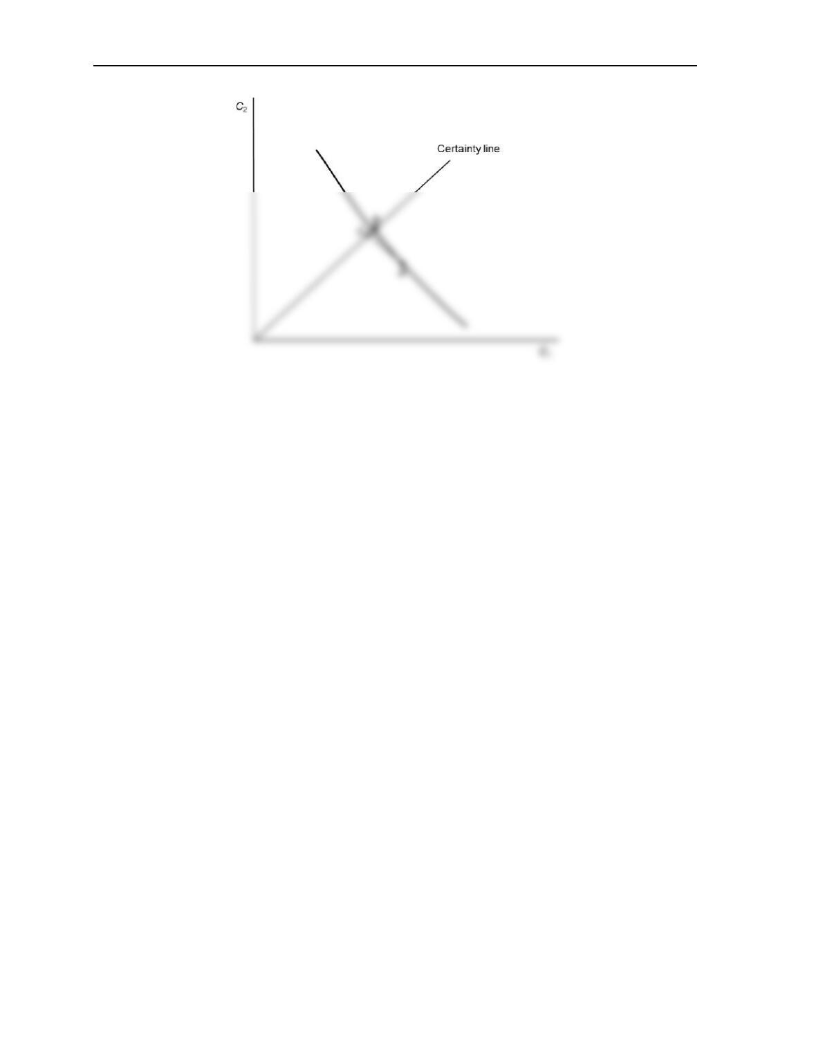
c. Return to the graph from part a, but imagine that point A is quite close to B.
Next imagine magnifying the graph, shown below. The bend in Leah’s indif-
Chapter 4: Uncertainty
8