88 CHAPTER 4 | Economic Efficiency, Government Price Setting, and Taxes
2.5 You should disagree. The first part of the statement is correct, but second part is incorrect. If
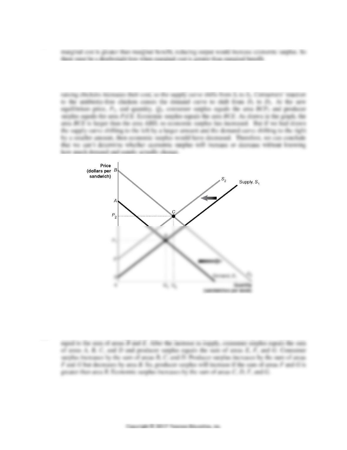
2.6 In the following graph, at the initial equilibrium price, P1, and quantity, Q1, consumer surplus
equals the area ABP1 and producer surplus equals the area P1BD. Economic surplus equals
consumer surplus plus producer surplus and is represented by the area ABD. The new method of
2.7 You should disagree. Consumer surplus may increase at the same time producer surplus increases
if an economy moves toward greater economic efficiency. The increased consumer surplus may
be due to a decrease in deadweight loss. Also, consumer surplus and producer surplus would both
increase if there was an increase in demand, holding everything else constant.
2.8 Before the increase in supply, consumer surplus was equal to area A and producer surplus was
CHAPTER 4 | Economic Efficiency, Government Price Setting, and Taxes 89
2.9 You should disagree. Economic surplus increases as long as marginal benefit exceeds marginal
cost for each additional unit of output. Economic surplus is greatest when the marginal benefit to
4.3
Government Intervention in the Market: Price Floors and Price Ceilings
Learning Objective: Explain the economic effect of government-imposed price floors
and price ceilings.
Review Questions
3.1 Some consumers gain from price controls because they can buy a product at a lower price, but
3.2 Producers tend to favor price floors that are set above the equilibrium price, but only if
producer surplus rises—as would be the case when the price rises a lot as a result of the price
3.3 A black market is one in which buyers and sellers violate government price regulations. A black
3.4 Economic analysis will show the trade-offs involved from imposing price ceilings and price
floors, but it won’t provide a final answer to the appropriateness of the policy because people
Problems and Applications
3.5 a. 28 million crates
b. A surplus of 6 million crates (QD = 28, QS = 34, Surplus = QS – QD = 34 – 28 = 6 million crates)
90 CHAPTER 4 | Economic Efficiency, Government Price Setting, and Taxes
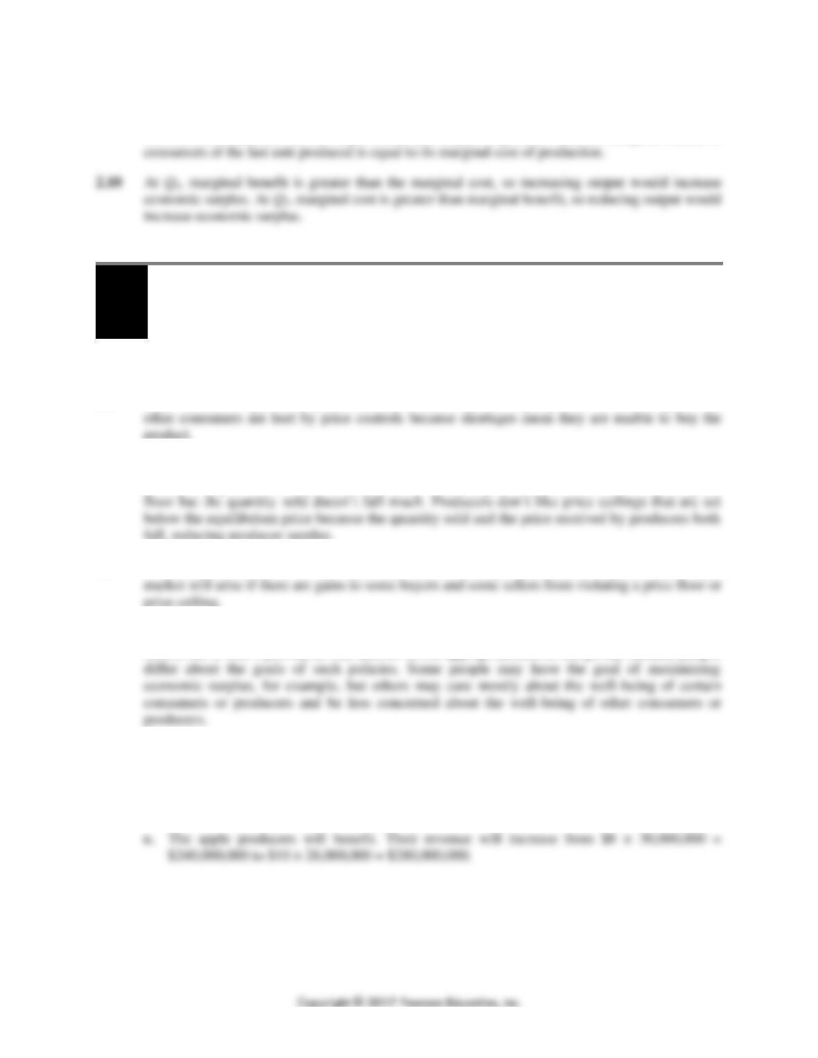
3.6 a. The equilibrium quantity is 100 million crates of kumquats per year and the equilibrium price
is $20 per crate. Kumquat producers receive revenue of $2 billion.
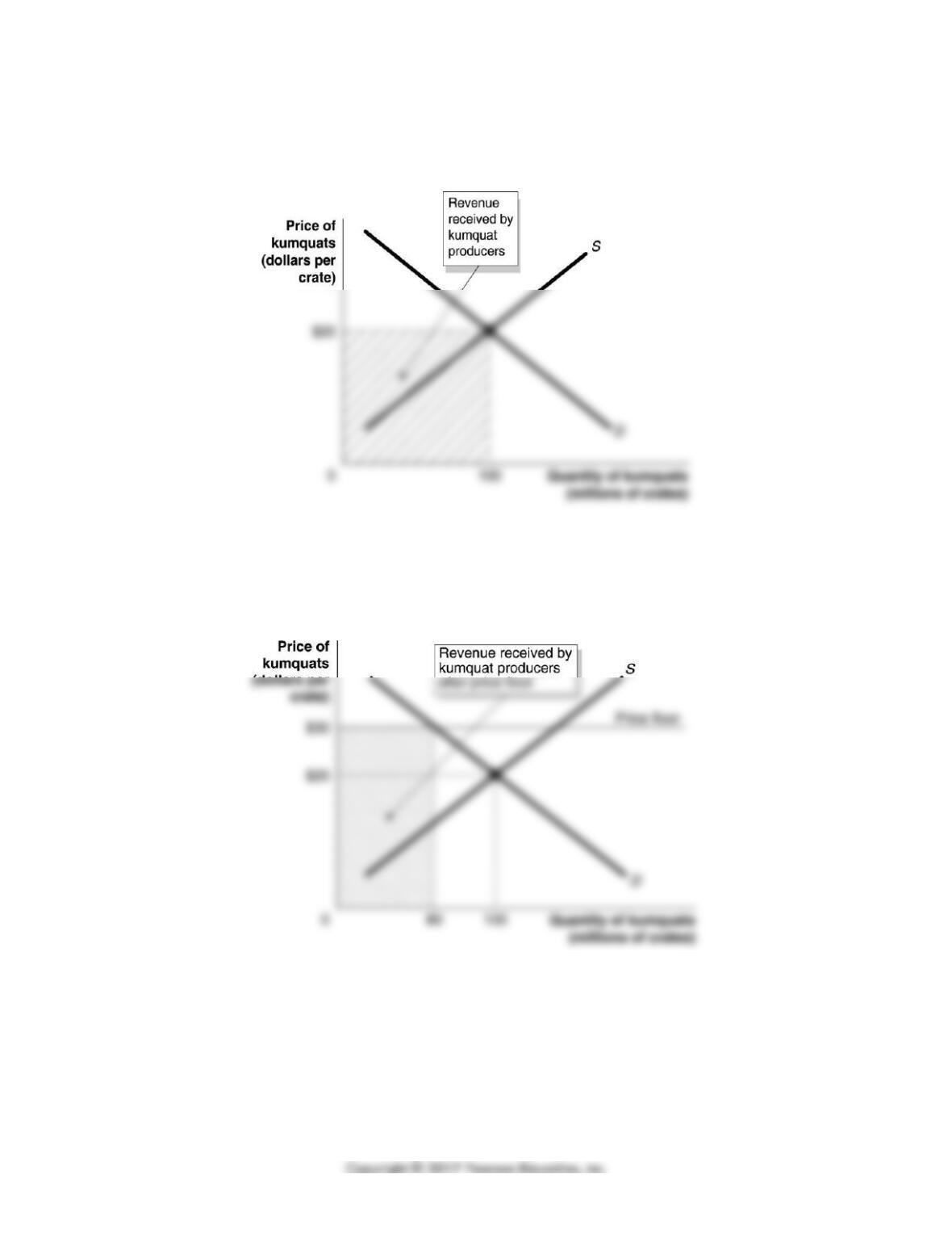
b. Consumers will purchase 80 million crates of kumquats. Kumquat producers receive revenue
of $2.4 billion: $30 × 80,000,000 = $2,400,000,000.
CHAPTER 4 | Economic Efficiency, Government Price Setting, and Taxes 91
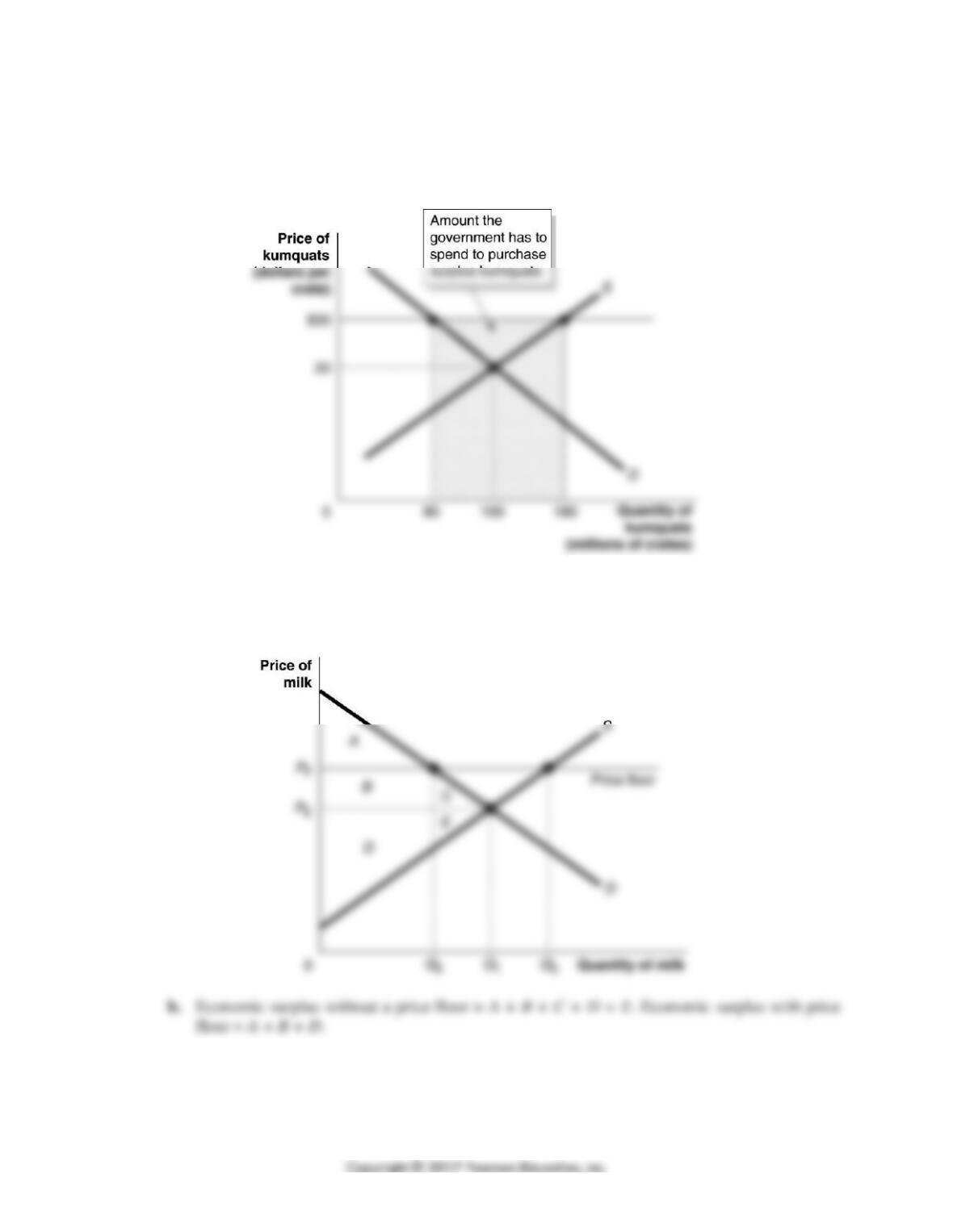
c. Kumquat producers will receive the revenue of $2.4 billion in part (b) plus $30 × 100 million
crates, or $3.0 billion, for a total of $5.4 billion. The government will spend $3.0 billion
purchasing the 100 million crates of surplus kumquats. Or we can calculate directly the total
amount kumquat producers will receive as $30 × 180 million crates = $5.4 billion.
3.7 a. PE is the competitive equilibrium price. PF is the price floor. Q1 is the quantity sold in
competitive equilibrium. Q2 is the quantity sold with the price floor.
92 CHAPTER 4 | Economic Efficiency, Government Price Setting, and Taxes
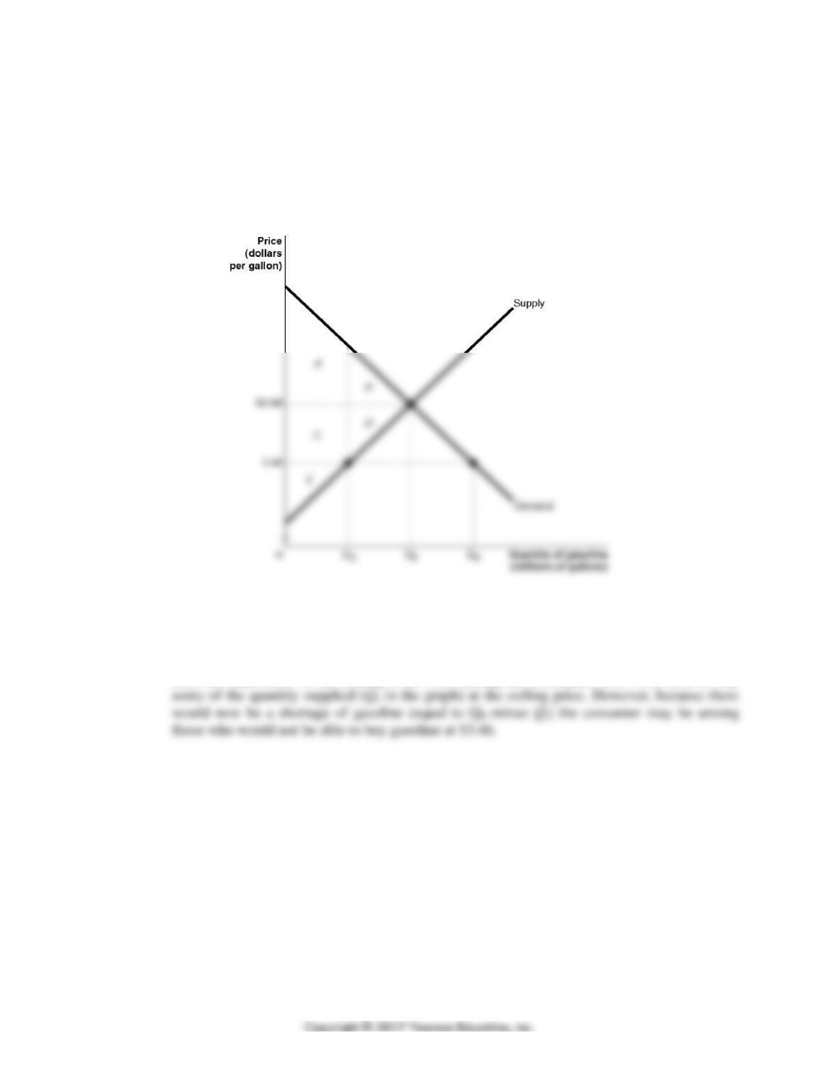
3.8 a. The following graph illustrates the effect of the price ceiling on the market for gasoline.
Prior to the imposition of the ceiling, consumer surplus would be equal to the sum of the
areas A and B. Producer surplus would equal the sum of areas C, D, and E. After the
imposition of the price ceiling consumer surplus would equal the sum of areas A and C;
producer surplus would equal area E. The ceiling would create a deadweight loss equal to
the sum of areas B and D.
b. The consumer who complained about the increase in the price of gasoline would be better off
after the imposition of the ceiling if he were among the consumers who were able to buy
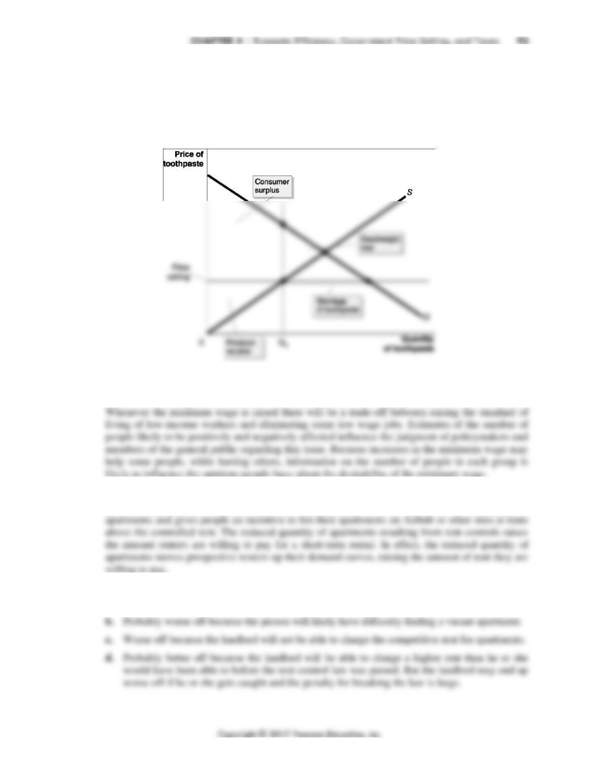
3.9 a. Price controls that make goods more affordable are price ceilings, which create shortages for
the goods.
b. As shown in the graph below, the price ceiling causes a shortage for toothpaste and leads to a
deadweight loss.
3.10 Raising the minimum wage would increase the incomes of people who had minimum wage jobs
previously, perhaps enough to lift them above the poverty line. But employers are unlikely to hire
those who they expect to contribute less than $10.10 of revenue per hour to their businesses.
3.11 If San Francisco repealed its rent control law, the prices for short-term rentals in San Francisco
listed on Airbnb and other peer-to-peer sites would likely fall. Rent control causes a shortage of
3.12 a. If someone is currently a renter, the law will probably make him or her better off, unless the
landlord decides to remove the apartment from the market.
94 CHAPTER 4 | Economic Efficiency, Government Price Setting, and Taxes
3.13 The statement is correct. If a good is not scarce (there is more freely available at a zero price than
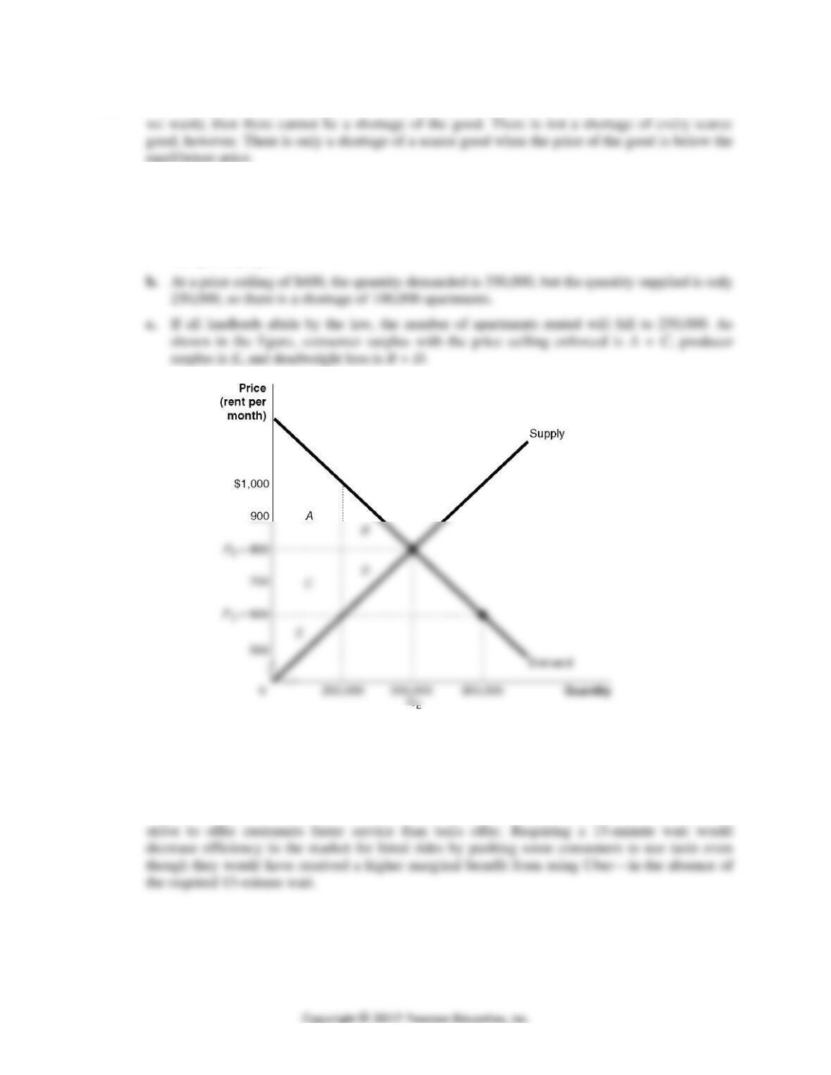
3.14 a. In the absence of rent control, the equilibrium price is $800, and the equilibrium quantity is
300,000. In this case, every renter who is willing to pay the market price of $800 will find an
apartment, and every landlord willing to accept the market price of $800 will find a renter.
The demand and supply curves are shown in the figure, along with the equilibrium price (PE)
and quantity (QE).
d. If landlords supply only 250,000 apartments and ignore the price ceiling, they can charge
$1,000; $1,000 is the highest rent that consumers are willing to pay to rent 250,000
apartments.
3.15 The insistence on a 15 minute wait between the time a passenger books a car and when he or she
is picked may seem odd, but taxi drivers fear competition from other services–such as Uber–that
CHAPTER 4 | Economic Efficiency, Government Price Setting, and Taxes 95
3.16 The first sentence of the student’s argument is correct. The second sentence is incorrect. A price
ceiling increases the quantity that consumers demand, but because it also reduces the quantity that
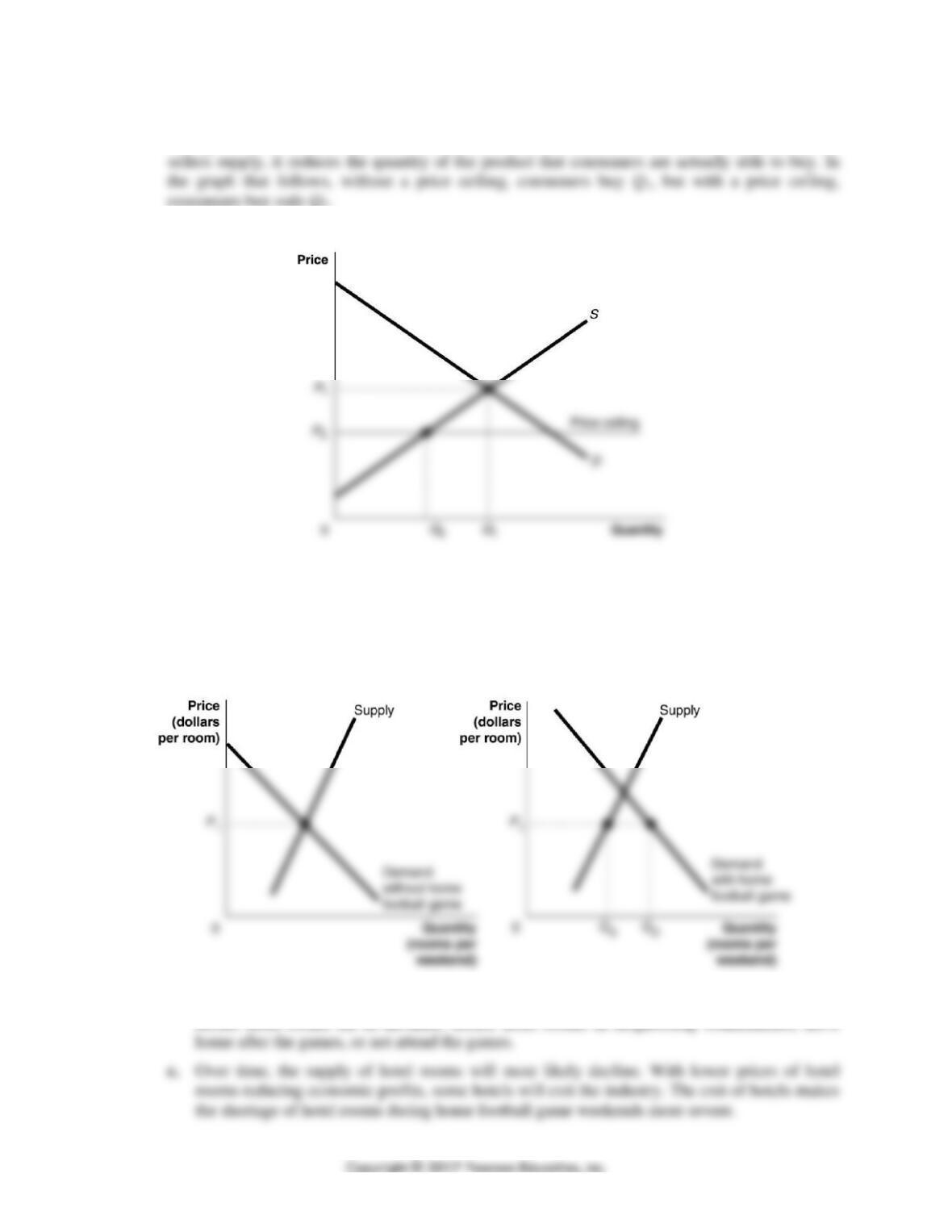
3.17 a. The demand for hotels rooms, shown in the figure below, increases during home football
games. If prices for rooms are not allowed to rise above P1, which is the equilibrium price
during weekends without home football games, during weekends with home football games
there will be a shortage of hotel rooms equal to QD minus QS.
b. Out-of-town footballs fans will have trouble finding a hotel room. They will have to try to
secure hotel rooms far in advance, secure hotel rooms in neighboring communities, drive
96 CHAPTER 4 | Economic Efficiency, Government Price Setting, and Taxes
d. Ski resorts and vacation spots have peak seasons. Laws limiting the prices hotels can charge
businesses.
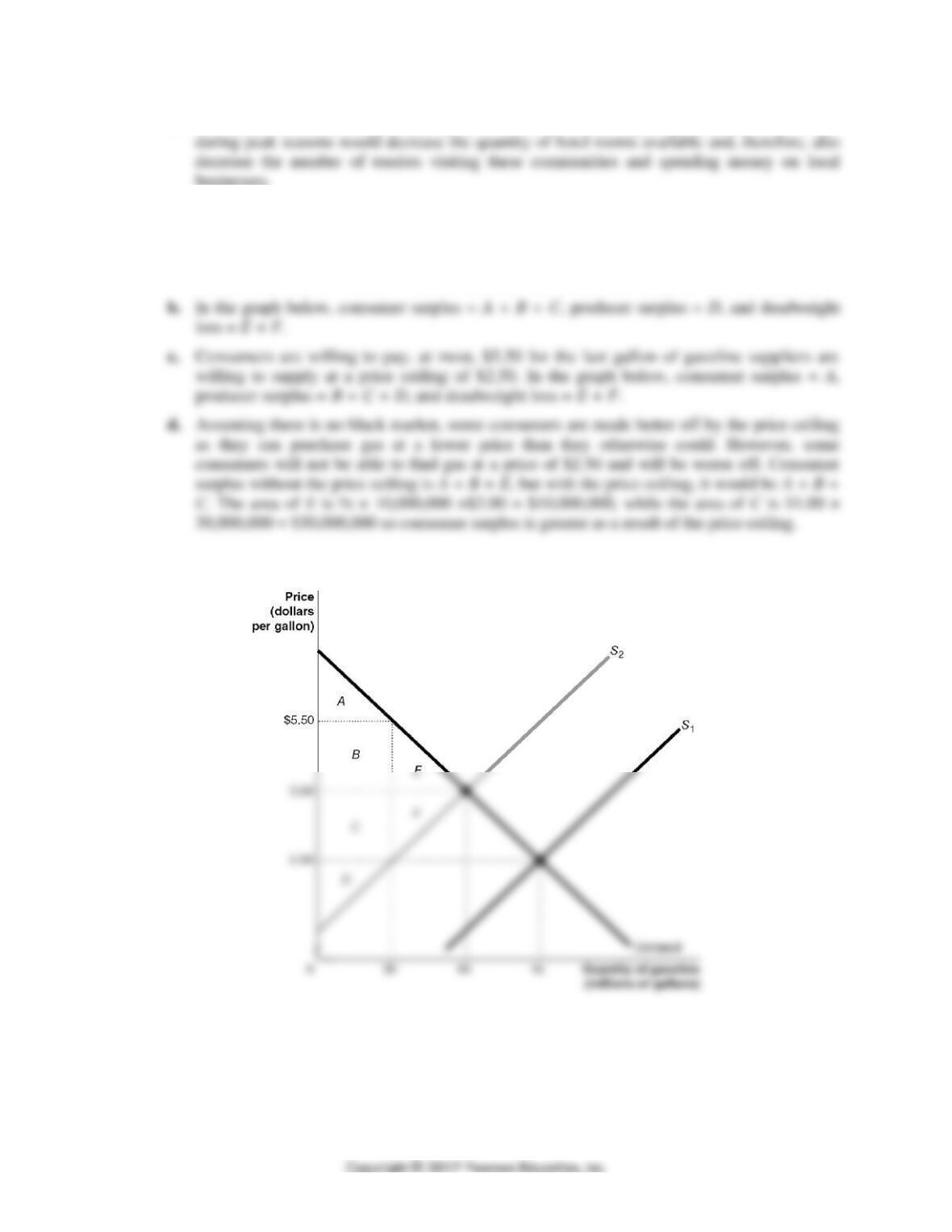
3.18 a. After the decrease in supply, with no price ceiling, the equilibrium price would be $3.50, and
the equilibrium quantity would be 40 million gallons. With a price ceiling of $2.50 and no
black market, the price will be $2.50, the quantity demanded will be 45 million gallons, and
the quantity supplied will be 30 million gallons, resulting in a shortage of 15 million gallons.
CHAPTER 4 | Economic Efficiency, Government Price Setting, and Taxes 97
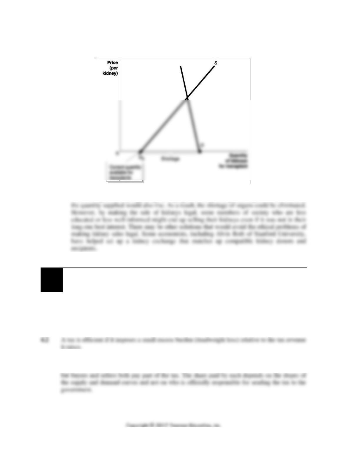
3.19 a.
b. Whether the government should allow the market to determine the price of kidneys is a
normative question. By legalizing the buying and selling of organs, the price would rise, and
4.4
The Economic Impact of Taxes
Learning Objective: Analyze the economic impact of taxes.
Review Questions
4.1 Tax incidence refers to the actual division of the burden of a tax between buyers and sellers in
a market.
4.3 The person who officially sends the tax revenue to the government need not be the one who
actually bears the burden of the tax. For most taxes, the seller sends the money to the government,
98 CHAPTER 4 | Economic Efficiency, Government Price Setting, and Taxes
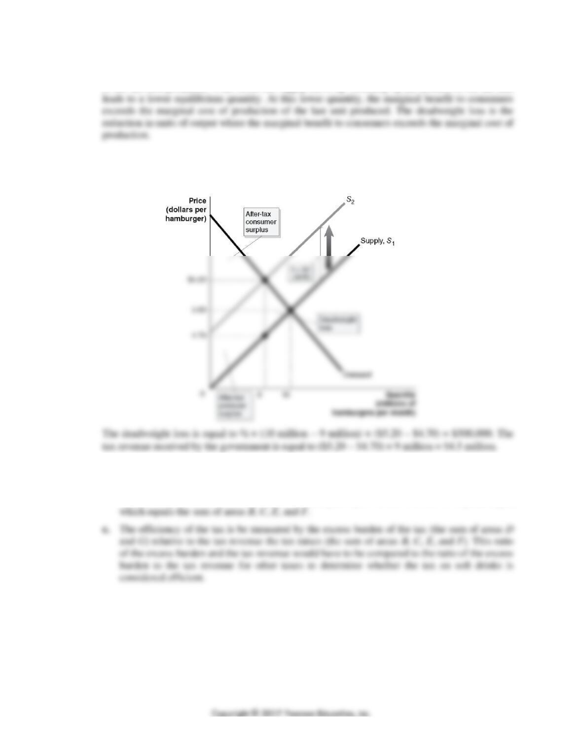
4.4 In market equilibrium, the marginal benefit to consumers equals the marginal cost of production
of the last unit produced. A tax shifts the supply curve up vertically by the amount of the tax and
Problems and Applications
4.5
4.6 a. The sum of areas D and G represent the excess burden (deadweight loss) of the tax.
b. The revenue collected by the government from the tax equals the amount of the tax (the
vertical distance between S1 and S2) times the quantity sold after the tax is imposed (Q2),
CHAPTER 4 | Economic Efficiency, Government Price Setting, and Taxes 99
4.7 a. The tax is $1.25 per pack, which is represented by the vertical distance between S1 and S2.
b. Producers receive $4.25 per pack.
c. The government receives tax revenues of $1.25 tax per pack × 18 billion packs = $22.5
billion a year.
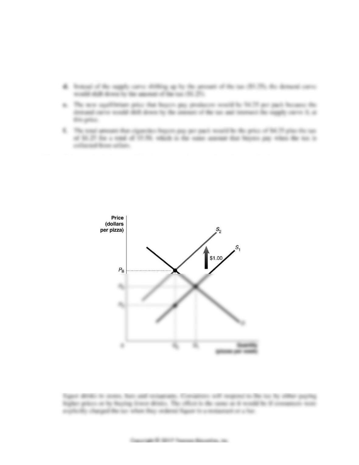
4.8 This reasoning is incorrect. The demand curve for pizzas slopes downward, and the supply curve
slopes upward, just as in other industries. So, as shown in the figure the tax will be split between
the buyers and sellers. The tax shifts the supply curve up from S1 to S2. The price paid by the
buyers increases from PE to PB, while the after-tax price received by the suppliers decreases from
PE to PS. PB – $1 = PS.
4.9 Although the tax on liquor is imposed on sellers, the tax can be viewed as would any increase in
the cost of production; that is, it will decrease supply and increase the price of wine and other
100 CHAPTER 4 | Economic Efficiency, Government Price Setting, and Taxes
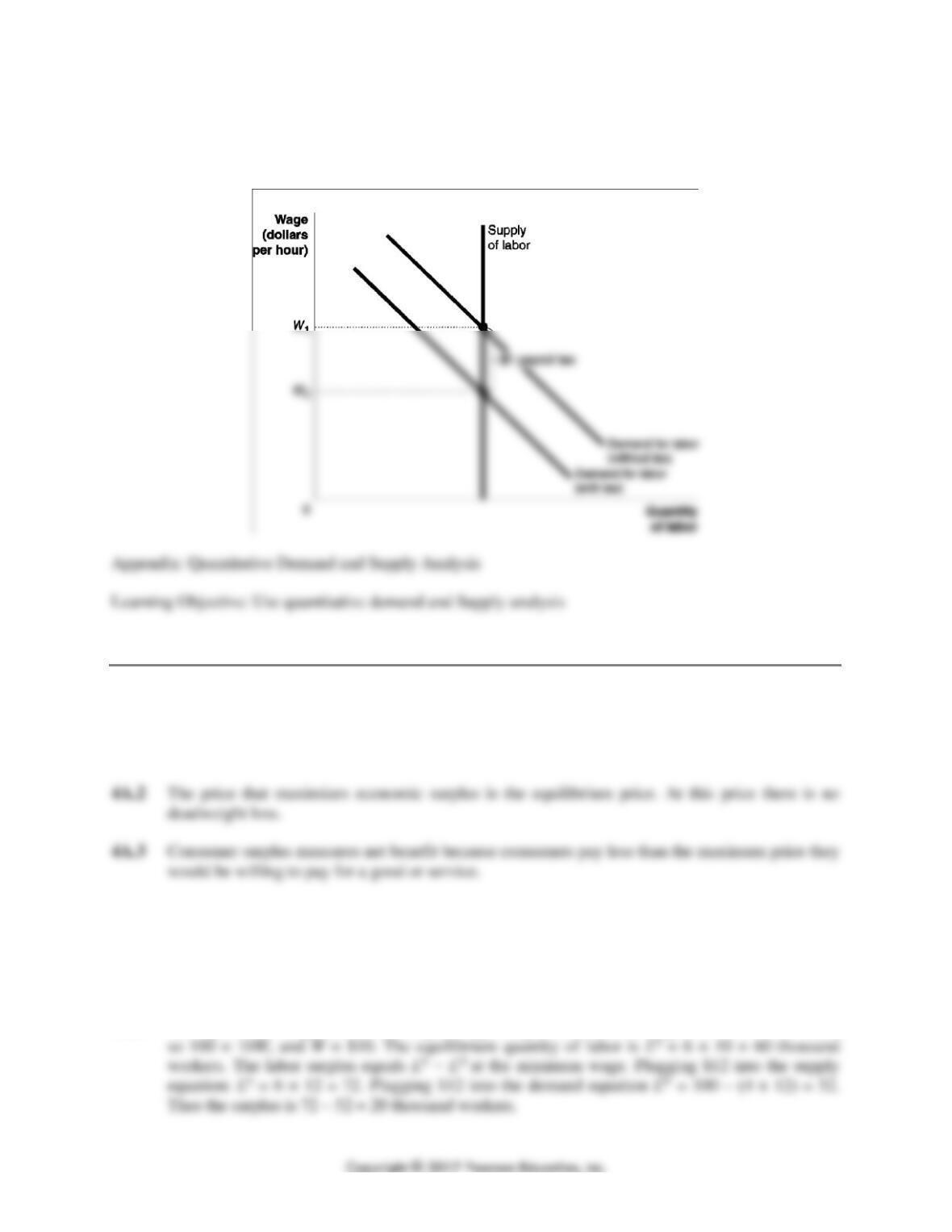
4.10 The $1 per hour of work payroll tax decreases the demand for labor by $1 at every quantity of labor.
With a vertical supply curve for labor, the wage rate drops by the full $1 tax. Workers bear the full
burden of the payroll tax. In the graph below, the equilibrium wage declines by $1 from W1 to W2.
Solutions to Chapter 4 Appendix
4A.1 In a linear demand equation, the intercept on the price axis represents the price at which the
quantity demanded is zero. No consumer is willing to pay this price or above for the product. In a
linear supply equation, the intercept on the price axis represents the price at which the quantity
supplied is zero. No firm is willing to produce the good at this price or less.
4A.4 Deadweight loss measures a net loss of economic surplus: The gains to consumers and producers
that could have been realized but were lost as a result of a price control or other policy. Some
policies result in a gain in surplus for one group that is transferred from some other group. A
deadweight loss results in a loss of surplus by a group of producers and consumers that is not
offset by a gain in surplus by another group of consumers or producers.
4A.5 The equilibrium wage can be found by setting LD equal to LS and solving for W. 100 – 4W = 6W,
CHAPTER 4 | Economic Efficiency, Government Price Setting, and Taxes 101
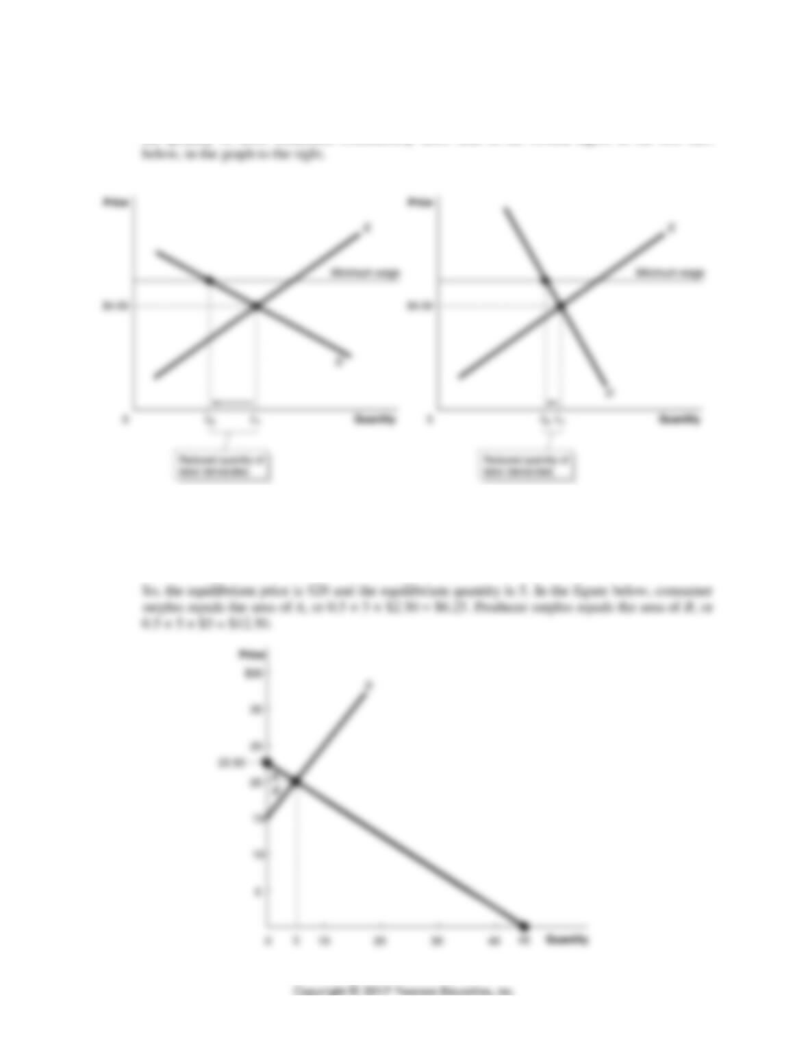
4A.6 The minimum wage will have a larger impact on employment in the top figure in the text and,
below, in the graph to the left. Because its demand curve is relatively flat, employers will reduce
the quantity of labor demanded considerably more than in the bottom figure in the text and,
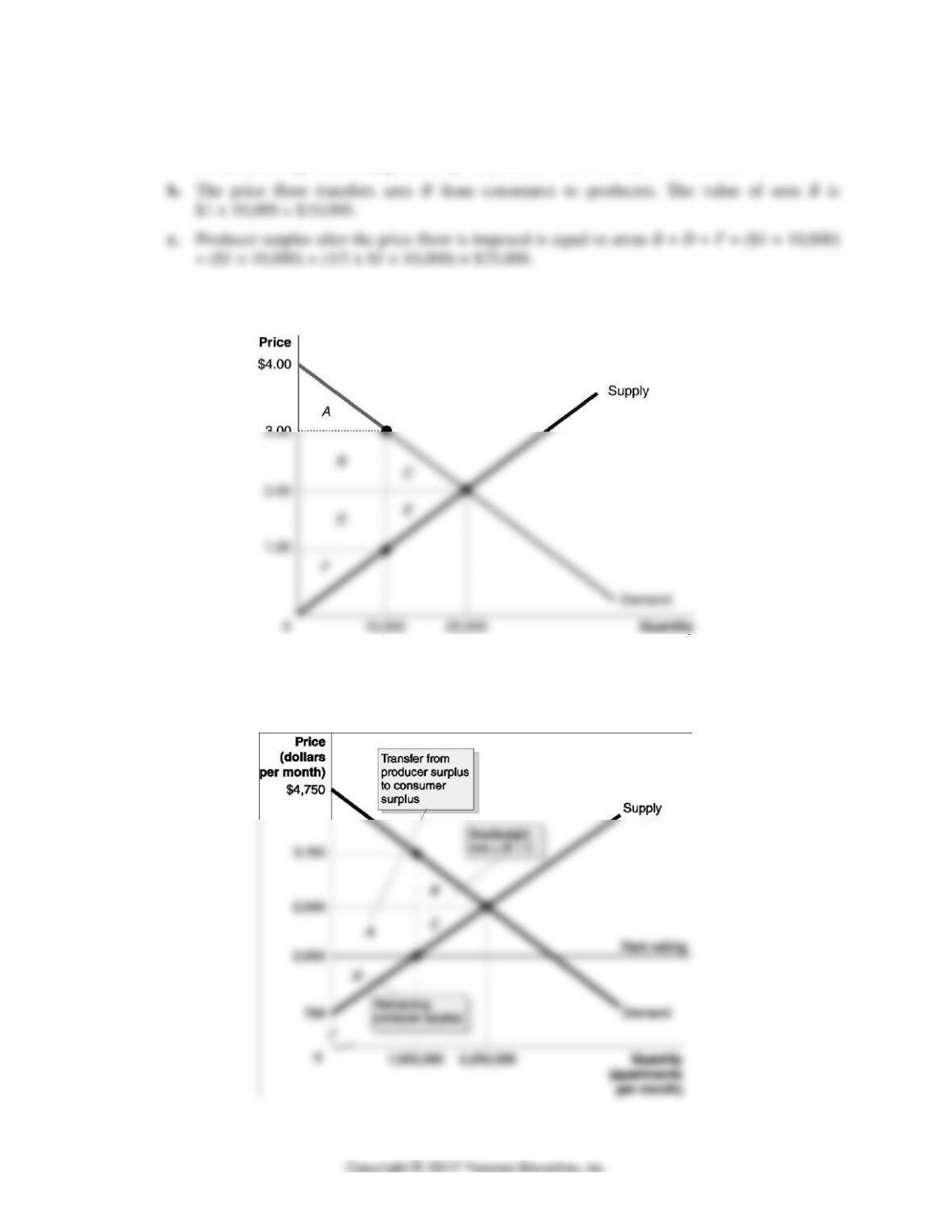
4A.7 We can use the fact that at equilibrium QD = QS to determine the equilibrium price and quantity:
45 − 2P = −15 + P
60 = 3P
P = $20, Q = 45 − 2(20) = 5
102 CHAPTER 4 | Economic Efficiency, Government Price Setting, and Taxes
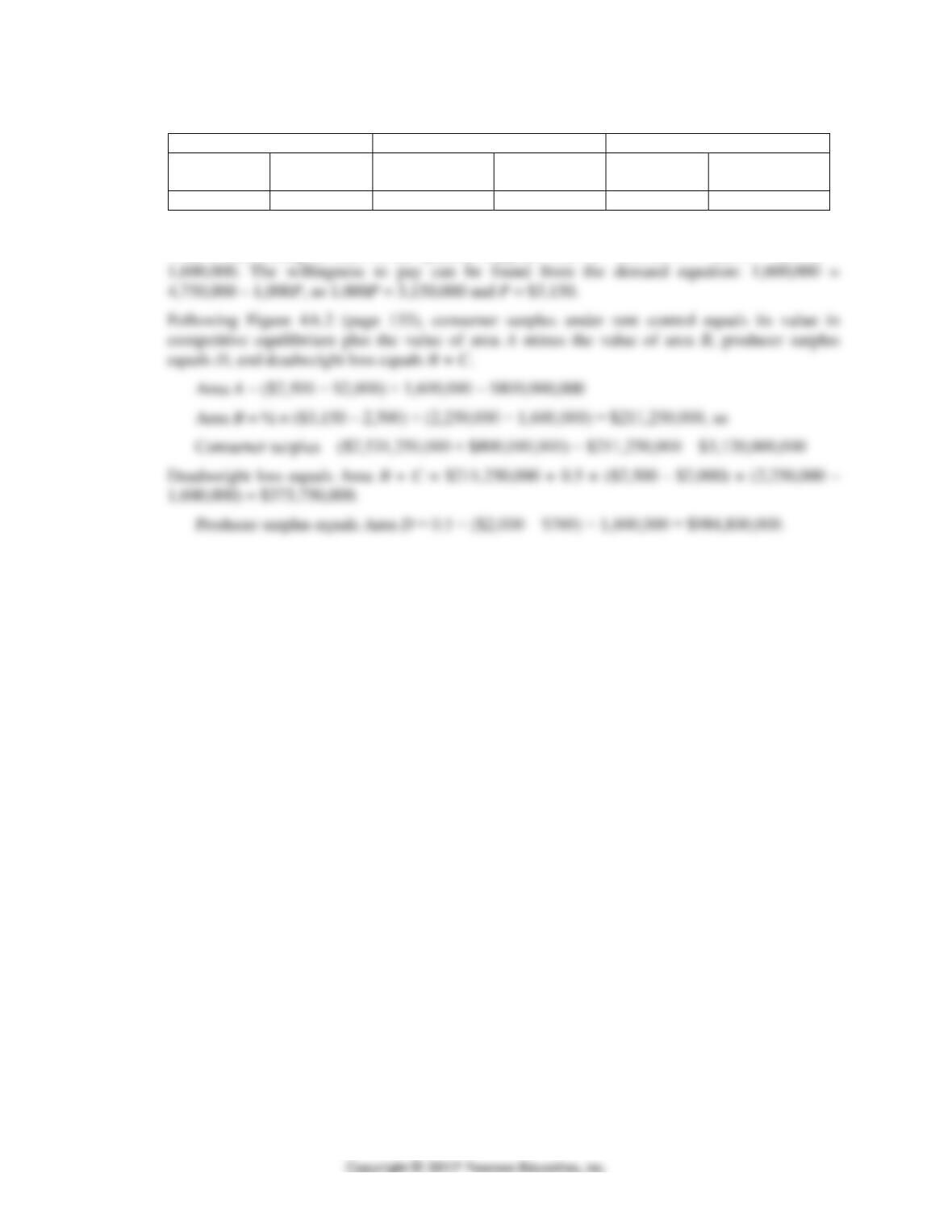
4A.8 a. The deadweight loss from the price floor equals C + E. C = 0.5 × $1 × 10,000 = $5,000 and
E = 0.5 × $1 × 10,000 = $5,000. So, deadweight loss = $10,000. Or, we can calculate the area
of the deadweight loss triangle directly: ½ (20,000 – 10,000) × (3 − 1) = $10,000.
d. Consumer surplus after the price floor is imposed is equal to area A. The value of area A is
½ × $1.00 × 10,000 = $5,000.
4A.9 The totals are in millions of dollars.
CHAPTER 4 | Economic Efficiency, Government Price Setting, and Taxes 103
Consumer surplus
Producer surplus
Deadweight loss
Competitive
equilibrium
Rent
control
Competitive
equilibrium
Rent
control
Competitive
equilibrium
Rent
control
$2,531
$3,120
$1,947
$985
$0
$374
With a rent ceiling of $2,000, the quantity supplied will be −1,000,000 + (1,300 × 2,000) =