Economics Chapter 4 The depreciation cost is the value lost as the capital

64 Chapter 4

5. The two components of the user cost of capital are the interest cost and the

depreciation cost. The depreciation cost is the value lost as the capital wears out

6. The desired capital stock is the amount of capital that allows the firm to earn the

largest possible profit. The higher the expected future marginal product of capital,

7. Gross investment represents the total purchase or construction of new capital

goods that takes place during a period. Net investment is gross investment minus

8. Equilibrium in the goods market occurs when the aggregate supply of goods (Y)

equals the aggregate demand for goods (Cd + Id + G). Since desired national

9. The saving curve slopes upward because saving is assumed to increase with an

increase in the expected real interest rate. The investment curve slopes downward

because investment is lower the higher is the expected real interest rate. The

Consumption, Saving, and Investment 65

NUMERICAL PROBLEMS

1. First, a general formulation of the problem is useful. With income of Y1 in the first

year and Y2 in the second year, the consumer saves Y2 – C in the first year and Y2

– C in the second year, where C is the consumption amount, which is the same in

both years. Saving in the first year earns interest at rate r, where r is the real

interest rate. And the consumer needs to accumulate just enough after two years

to pay for college tuition, in the amount T. So the key equation is (Y1 – C)(1 + r) +

(Y2 – C) = T.

a. Y1 = Y2 = $25 000, r = 10%, T = $6300. The key equation gives ($25 000 – C)

1.1 + ($25 000 – C) = $6300. This can be simplified to $25 000 – C =

$6300/2.1 = $3000, which can be solved to get C = $22 000. Then S = Y – C

= $25 000 – $22 000 = $3000.

d. With the increase in wealth of W, the total amount invested for the second

period is W + Y1 – C, so the key equation becomes ($525 + $25 000 – C)1.1

+ ($25 000 – C) = $6300. This can be simplified to ($25 525 × 1.1) + $25 000

66 Chapter 4

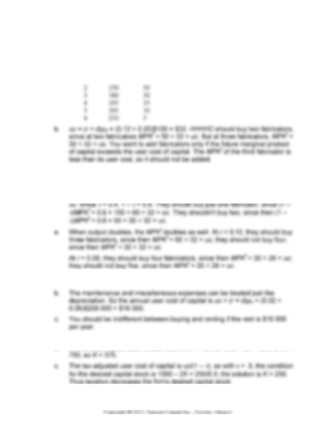
2. a. This chart shows the MPKf as the increase in output from adding another

fabricator.

# Fabricators Output MPKf

0 0 —

1 100 100

c. When r = 0.08, uc = (0.08 + 0.20)$100 = $28. Now they should buy three

fabricators, since MPKf = 30 > 28 = uc for the third fabricator and MPKf = 15 <

28 = uc for the fourth fabricator.

d. With taxes, they should add additional fabricators as long as (1 –

τ

)MPKf >

3. a. The expected after-tax real interest rate is r = i(1 –

τ

) – πe = 0.10 (1 – 0.30) –

0.05 = 0.07 – 0.05 = 0.02.

4. a. uc = (r + d)pK = (0.10 + 0.15)$1000 = $250.

b. The desired capital stock is such that MPKf = uc, so 1000 – 2K = 250, or 2K =

Consumption, Saving, and Investment 67

d. The investment tax credit basically lowers the price of capital from $1000 to (1

5. a. Desired consumption declines as the real interest rate rises because the

higher return to saving encourages higher saving; desired investment

declines as the real interest rate rises because the user cost of capital is

higher, reducing the desired capital stock, and thus investment.

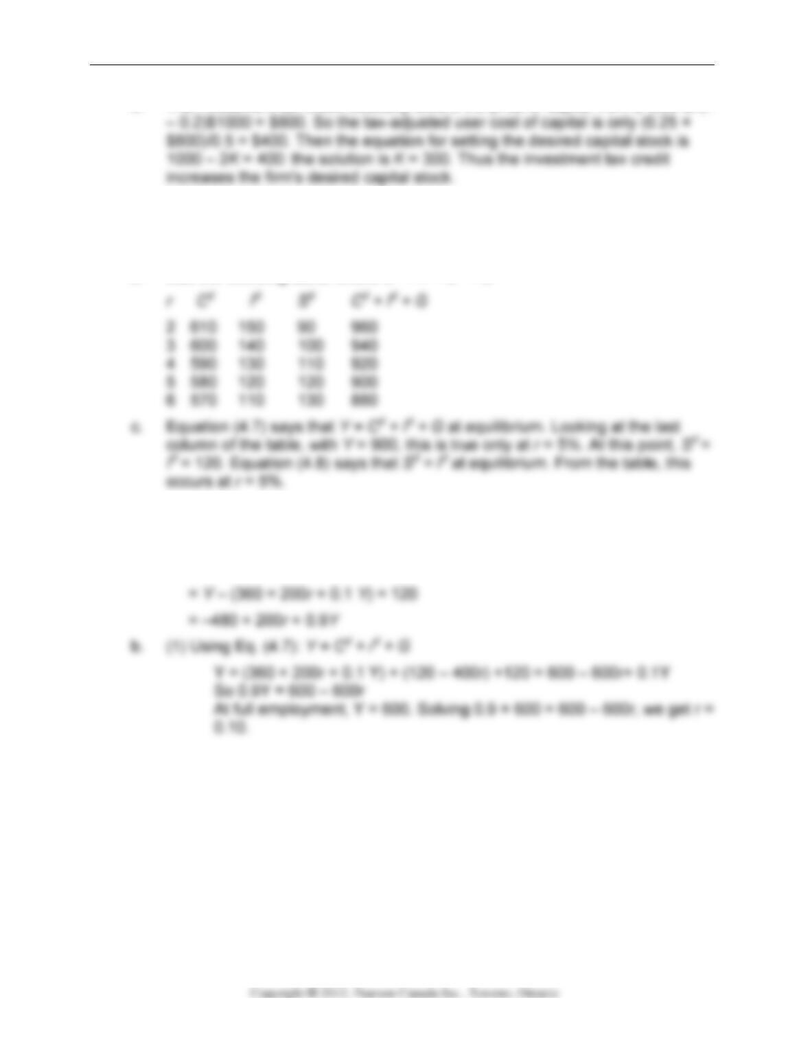
b. Use the following table, where Sd = Y – Cd – G

d. When government purchases fall by 40 to 160, each Sd entry in the table is

higher by 40, and each Cd + Id + G entry is lower by 40. Then Y = Cd + Id + G

occurs at r = 3%, as does Sd = Id = 140.

6. a. Sd = Y – C – G

68 Chapter 4

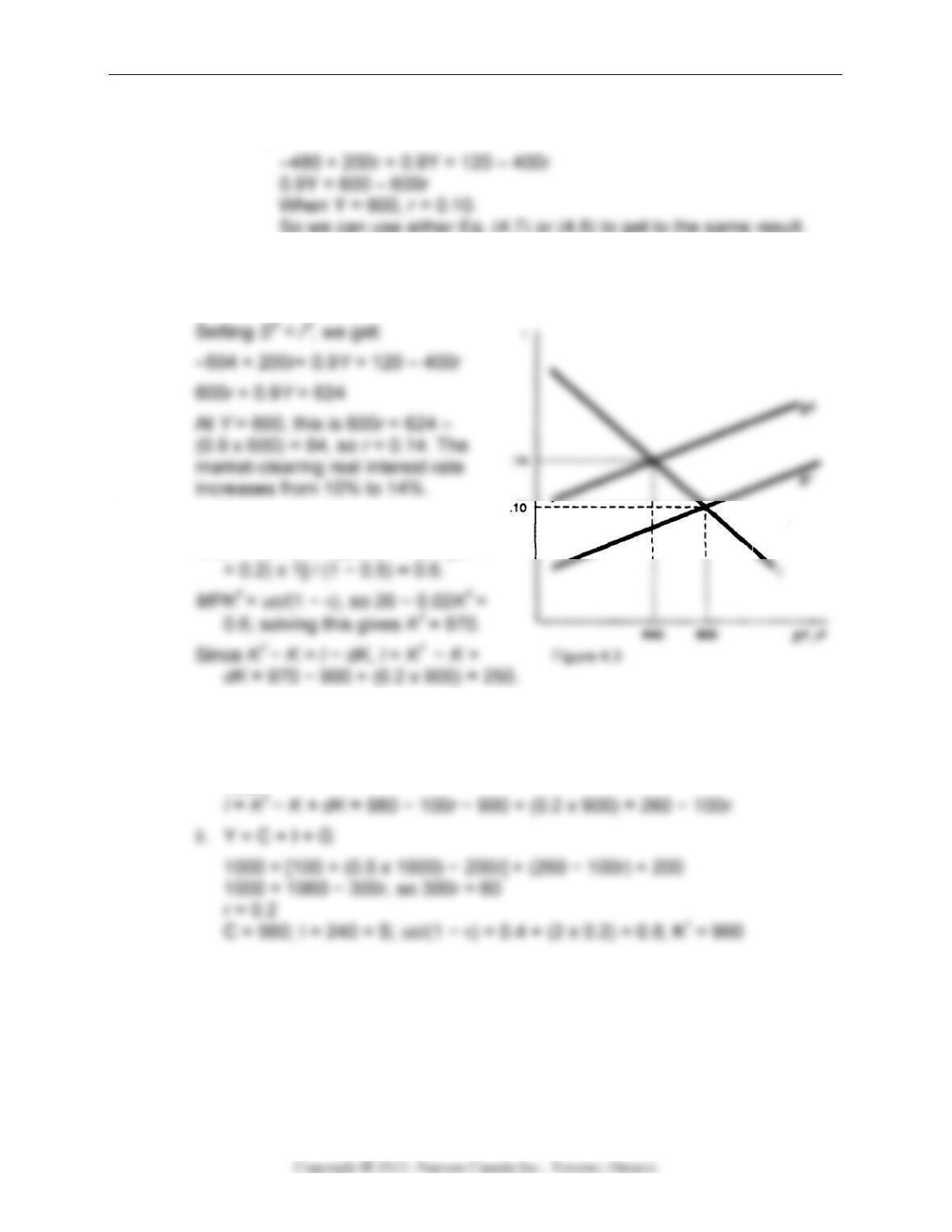
(2) Using Eq. (4.8): Sd = /d

So we can use either Eq. (4.7) or (4.8) to get to the same result.

c. When G = 144, desired saving becomes Sd = Y – Cd – G = Y – (360 – 200r +

0.1 Y) – 144 = –504 + 200r + 0.9Y. Sd is now 24 less for any given r and Y;

this shows up as a shift in the Sd line from S1 to S2 in Fig. 4.3.

7. a. r = 0.10

uc/(1 − τ) = (r + d)pK /(1 − τ) = [(0.1

b. i. Solving for this in general:

uc/(1 – τ) = (r + d)pK / (1 − τ) = [(r + 0.2) x 1] / (1 − 0.5) = 0.4 + 2r.

MPKf = uc/(1 − τ), so 20 − 0.02K = .4 + 2r; solving this gives Kf = 980 −

100r.

Consumption, Saving, and Investment 69

Analytical Problems

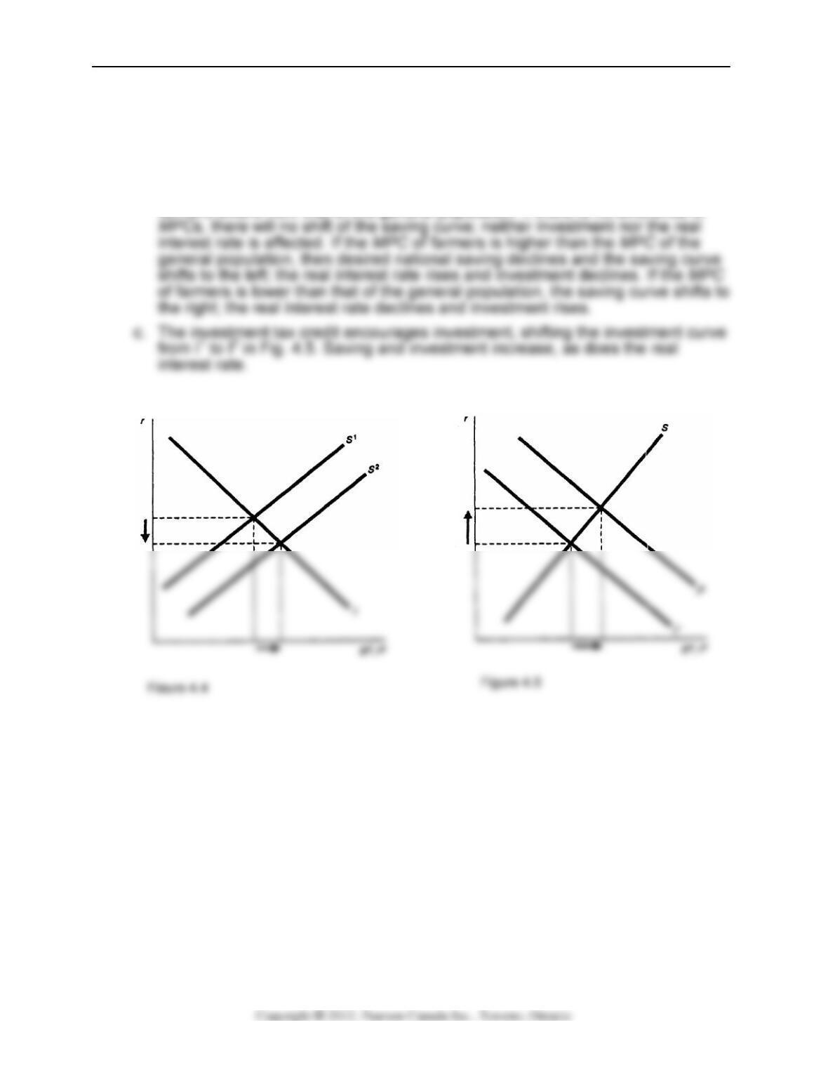
1. a. As Fig. 4.4 shows, the shift to the right in the saving curve from S1 to S2 causes

saving and investment to increase and the real interest rate to decrease.

b. This is really just a transfer from the general population to farmers. The effect

on saving depends on whether the marginal propensity to consume (MPC) of

farmers differs from that of the general population. If there is no difference in

70 Chapter 4

d. The increase in expected future income decreases current desired saving, as

people increase desired consumption immediately. The rise of the future

marginal productivity of capital shifts the investment curve to the right. The

result, as shown in Fig. 4.6, is that the real interest rate rises, with ambiguous

effects on saving and investment.

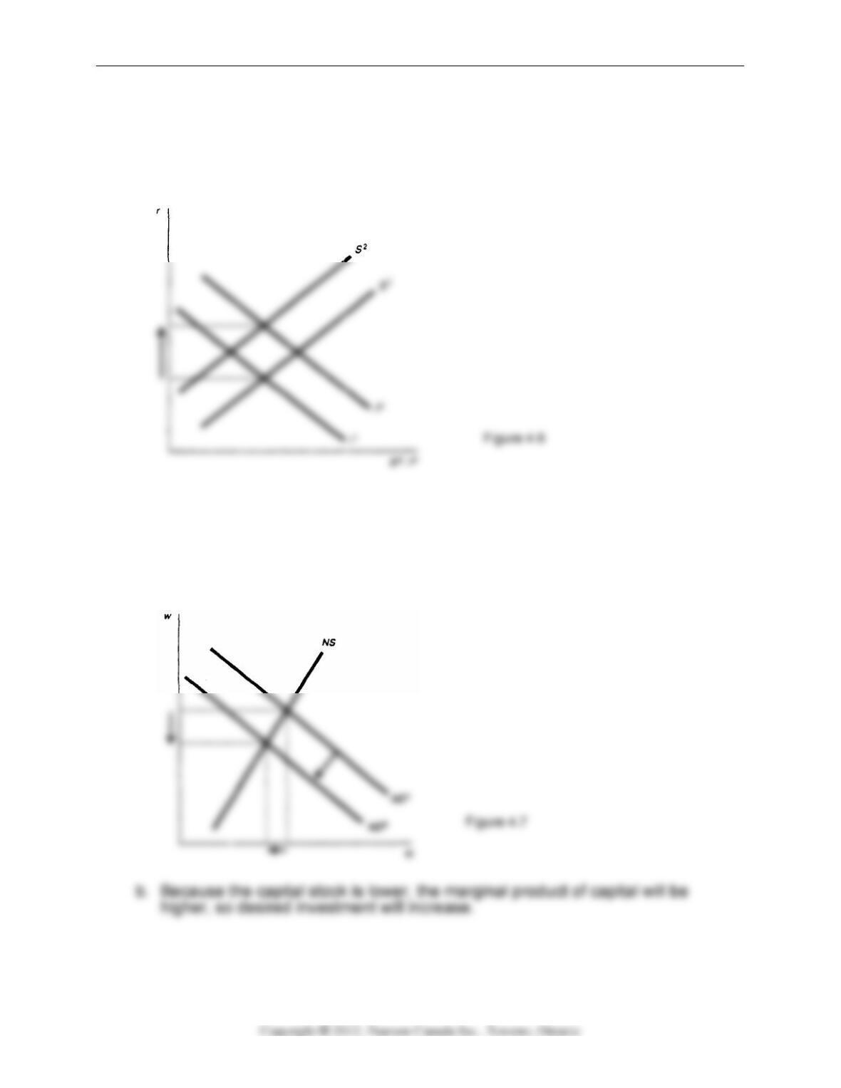
2. a. With a lower capital stock, the marginal product of labour is reduced, so the

labour demand curve shifts to the left from ND1 to ND2 in Fig. 4.7. Then the

new equilibrium point is one with lower employment and a lower real wage.

With lower employment and a lower capital stock, full-employment output will

be lower.

Consumption, Saving, and Investment 71

c. Since current output declines, desired saving declines, because people do not

want to reduce their consumption. On the other hand, since future output is also

lower, people desire to save more today to make up for the loss of future

income.

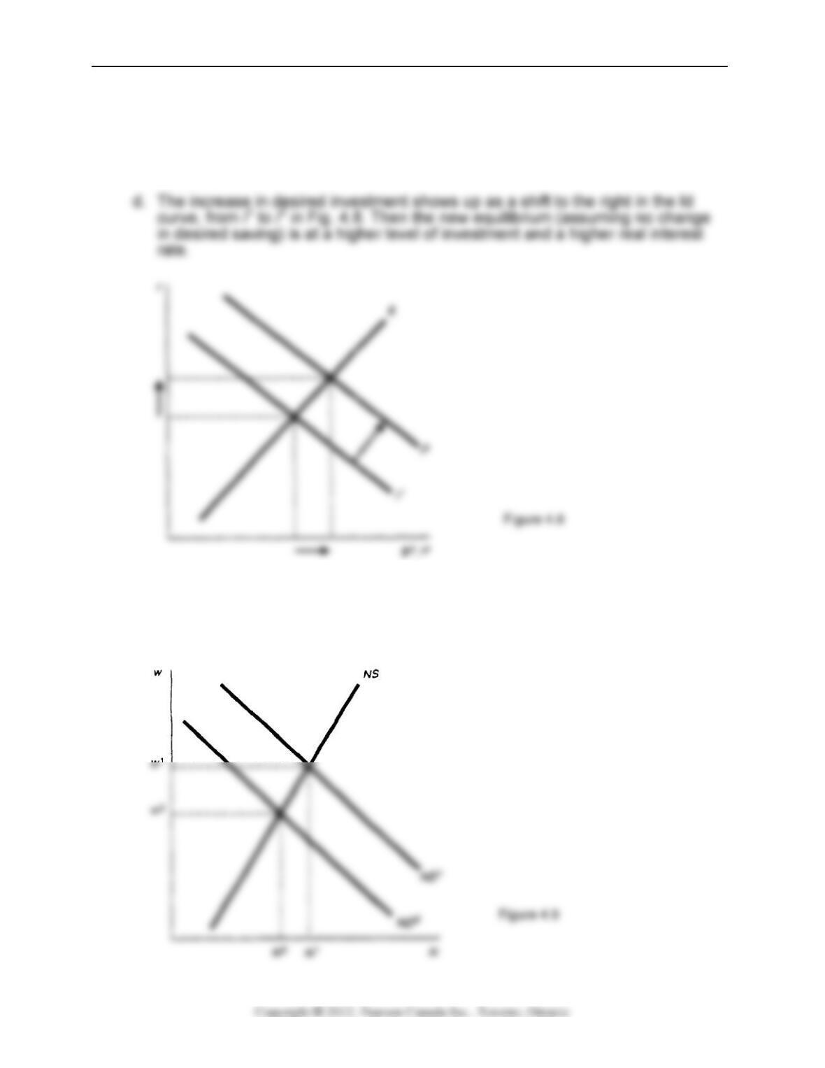
3. a. The temporary increase in the price of oil reduces the marginal product of

labour, causing the labour demand curve to shift to the left from ND1 to ND2 in

Fig. 4.9. At equilibrium, there is a reduced real wage and lower employment.

72 Chapter 4

The productivity shock results in a reduction of output. Because the shock is

temporary, the only effect on desired saving or investment is due to the

b. The permanent increase in the price of oil reduces the marginal product of

labour, causing the labour demand curve to shift to the left, again as in Fig. 4.9.

At equilibrium, there is a reduced real wage and lower employment.

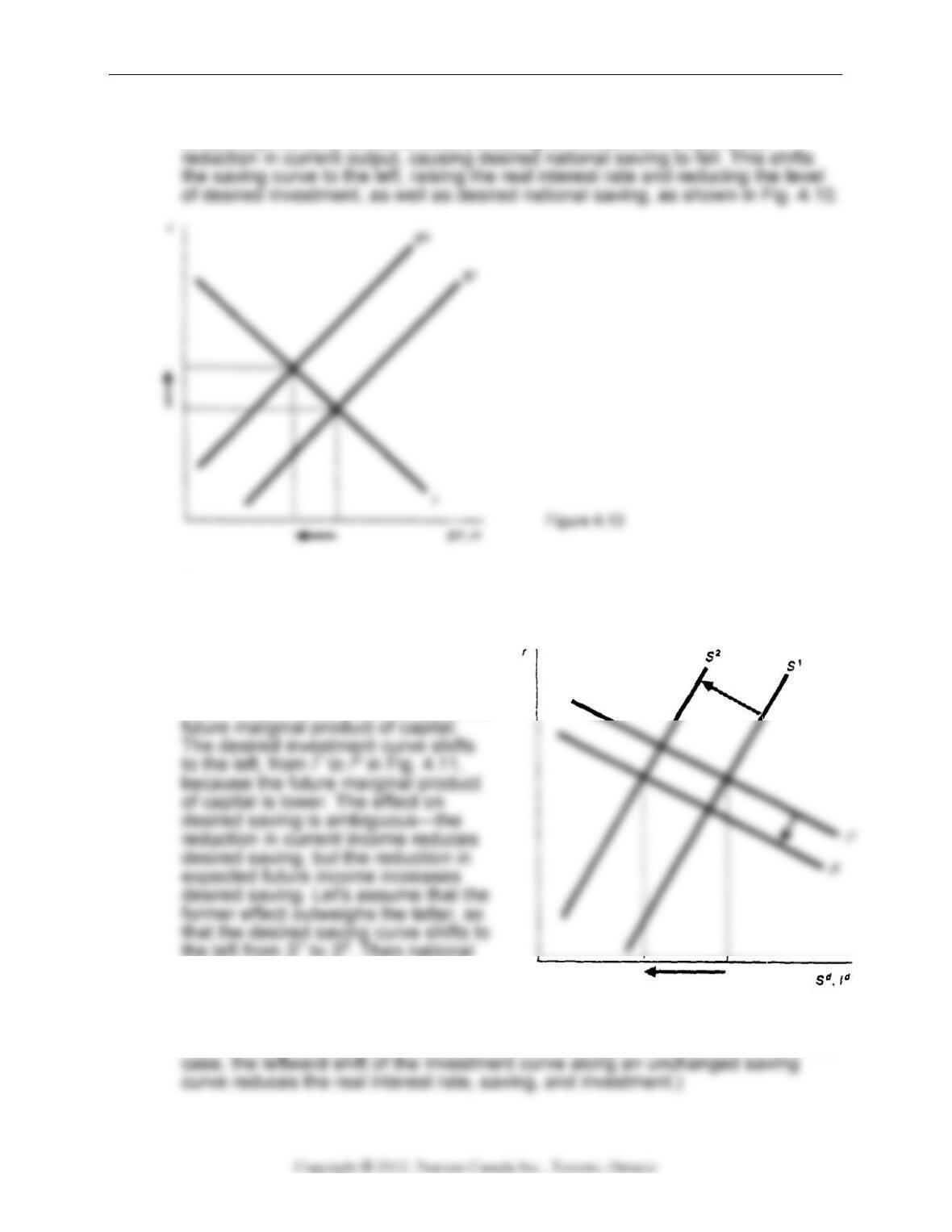
The productivity shock results in a

reduction of current output. Because

the shock is permanent, it reduces

future output as well, and reduces the

the left from S1 to S2. Then national

saving and investment both decline.

Again, the effect on the real interest

rate is ambiguous. (Alternatively, if

the effects on desired saving of the reductions in current income and future

income offset each other exactly, the desired saving curve does not shift, in this

Figure 4.11

Consumption, Saving, and Investment 73

4. A temporary increase in government spending reduces national saving. Whether

the spending is financed by current taxes or by borrowing (and raising future

taxes), consumption falls, but not by the full amount of the spending. Since S = Y –

Cd – G, national saving declines. This is shown in Fig. 4.12 as a shift to the left in

the saving curve. The real interest rate must increase to get S = /, so / declines as

well. It makes no difference whether the temporary increase in spending is funded

by taxes or by borrowing.

74 Chapter 4

5. When there is a temporary increase in government spending, consumers

foresee future taxes. As a result, consumption declines, both currently and in the

future. Thus current consumption does not fall by as much as the increase in G, so

national saving (Sd = Y – Cd – G) declines at the initial real interest rate, and the

When there is a permanent increase in government spending, consumers foresee

future taxes as well, with both current and future consumption declining. But if

there is an equal increase in current and future government spending, and

consumers try to smooth consumption, they will reduce their current and future

consumption by about the same amount, and that amount will be about the same