
CHAPTER 4
Consumer and Firm Behaviour: The Work–Leisure
Decision and Profit Maximization
KEY IDEAS IN THIS CHAPTER
2. The consumer’s optimizing consumption and leisure bundle is the one at which the
marginal rate substitution of leisure for consumption equals the real wage.
3. Assuming consumption and leisure are normal goods, an increase in the consumer’s
5. The representative firm’s goal is to hire the quantity of labour that maximizes her
profits.
7. The firm’s demand for labour curve is nothing but the marginal product of labour
NEW IN THE THIRD EDITION
1. All data and graphs have been updated.
2. New: “Macroeconomics in Action: How Elastic is Labor Supply?”
TEACHING GOALS
The microeconomic approach to macroeconomics stresses the notion that economy-wide
events are the result of decisions made by individuals. People work so that they may
afford to buy market goods. On the other hand, people generally prefer to work less rather
than work more. Although discussions in the popular press often refer to the idea that
spending is what drives the economy, an economy cannot produce unless people are

Instructor’s Manual for Macroeconomics, Fourth Canadian Edition
willing to work. Therefore, the most basic macroeconomic decision is to choose whether,
and how much, to work. Production and willingness to work are intrinsically
interconnected.
Students often believe that how much a person works is largely determined by the
necessities of their circumstances. Students will report that they have to work to survive
and pay tuition. Some students might point out that they need not work much or at all
Two key points of this chapter are the concepts of income and substitution effects. Often,
students are perplexed at the amount of time spent on this material because nothing in
practice is purely an income effect or a substitution effect. However, the two most basic
CLASSROOM DISCUSSION TOPICS
Ask students about their work choices and the choices of their parents, friends, and
relatives. Does everyone work? Does everyone work the same number of hours? Then
ask students for examples of the kinds of factors that lead people to work more or less.
Try to elicit very specific examples. Then ask students to categorize these factors that
lead to more or less work. Some of these factors are actually the byproducts of more
complex decision making. For example, if they say that they work more or less because
they go to school, point out that going to school is a choice. They may also point to
Ask students to provide examples of factors other than more labour or capital that can
allow some countries to be a lot more productive than others. What factors other than
growth in capital and labour allow a given economy to produce more (or less) over time?

Chapter 4: Consumer and Firm Behaviour: The Work–Leisure Decision and Profit Maximization
OUTLINE
1. The Representative Consumer
a) Consumer’s Preferences
i) The Consumption Good and Leisure
ii) The Utility Function
(2) Preference for Diversity
(1) Downward Sloping
(2) Convex to the Origin
iv) Marginal Rate of Substitution
b) Consumer’s Budget Constraint
i) Price-Taking Behaviour
ii) The Time Constraint
iii) Real Disposable Income
iv) The Budget Constraint
v) A Graphical Representation
c) Consumer Optimization
i) Rational Behaviour
ii) The Optimal Consumption Bundle
iii) Marginal Rate of Substitution = Relative Price
iv) A Graphical Representation
2. The Representative Firm
a) The Production Function
i) Constant Returns to Scale
ii) Monotonicity
iii) Declining MPN
iv) Declining MPK
v) Changes in Capital and MPN
Instructor’s Manual for Macroeconomics, Fourth Canadian Edition
b) Total Factor Productivity
c) Henry Ford and Total Factor Productivity (Macroeconomics in Action 4.1)
e) The Profit Maximization Problem of the Representative Firm
i) Profits = Total Revenue − Total Variable Costs
TEXTBOOK QUESTION SOLUTIONS
Problems
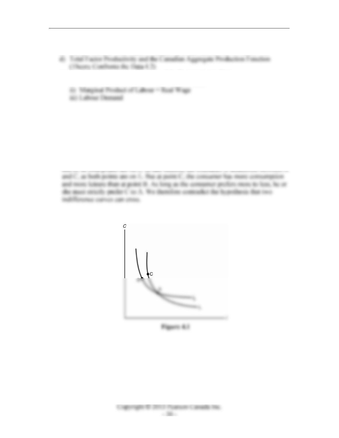
1. Consider the two hypothetical indifference curves in Figure 4.1. Point A is on both
indifference curves, I1 and I2. By construction, the consumer is indifferent between A
Chapter 4: Consumer and Firm Behaviour: The Work–Leisure Decision and Profit Maximization
2. ualbC=+
a) To specify an indifference curve, we hold utility constant at u. Next rearrange in
the form:
ua
Cl
bb
=−
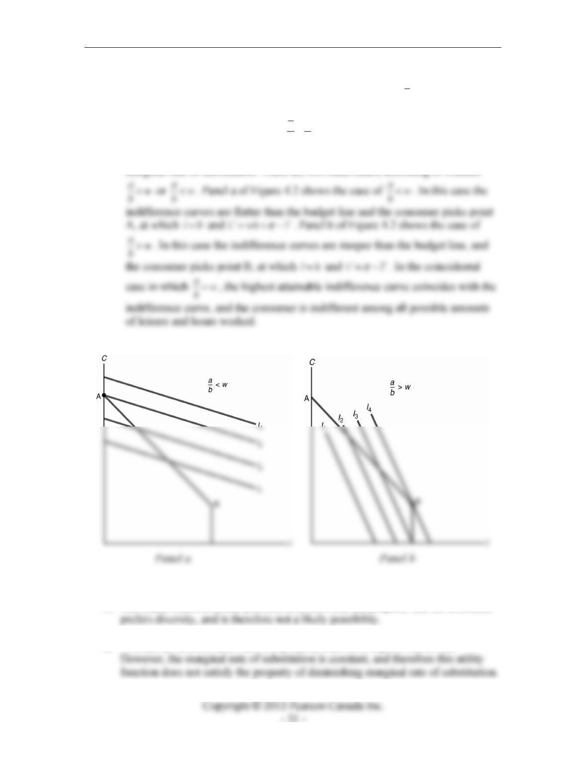
Indifference curves are therefore linear with slope, –a/b, which represents the
marginal rate of substitution. There are two main cases, according to whether
Figure 4.2
b) The utility function in this problem does not obey the property that the consumer
c) This utility function does have the property that more is preferred to less.

3. Suppose that h = 16. Then, the budget constraint for the consumer is
,68)16(75. −+−= lC
and since perfect complements with a =1 implies that the consumer wishes to
equalize leisure and consumption, this gives C = l. Then, substituting in the above
4. When the government imposes a proportional tax on wage income, the consumer’s
budget constraint is now given by:
(1 )( ) ,Cw thl T
π
=− −+−
where t is the tax rate on wage income. In Figure 4.3, the budget constraint for t = 0 is
FGH. When t > 0, the budget constraint is EGH. The slope of the original budget line
is –w, while the slope of the new budget line is –(1 – t)w. Initially the consumer picks
point A on the original budget line. After the tax has been imposed, the consumer
The tax also makes the consumer worse off, in that he or she can no longer be on
indifference curve I1, but must move to the less preferred indifference curve, I2. This
pure income effect moves the consumer to point B, which has less consumption and
Chapter 4: Consumer and Firm Behaviour: The Work–Leisure Decision and Profit Maximization
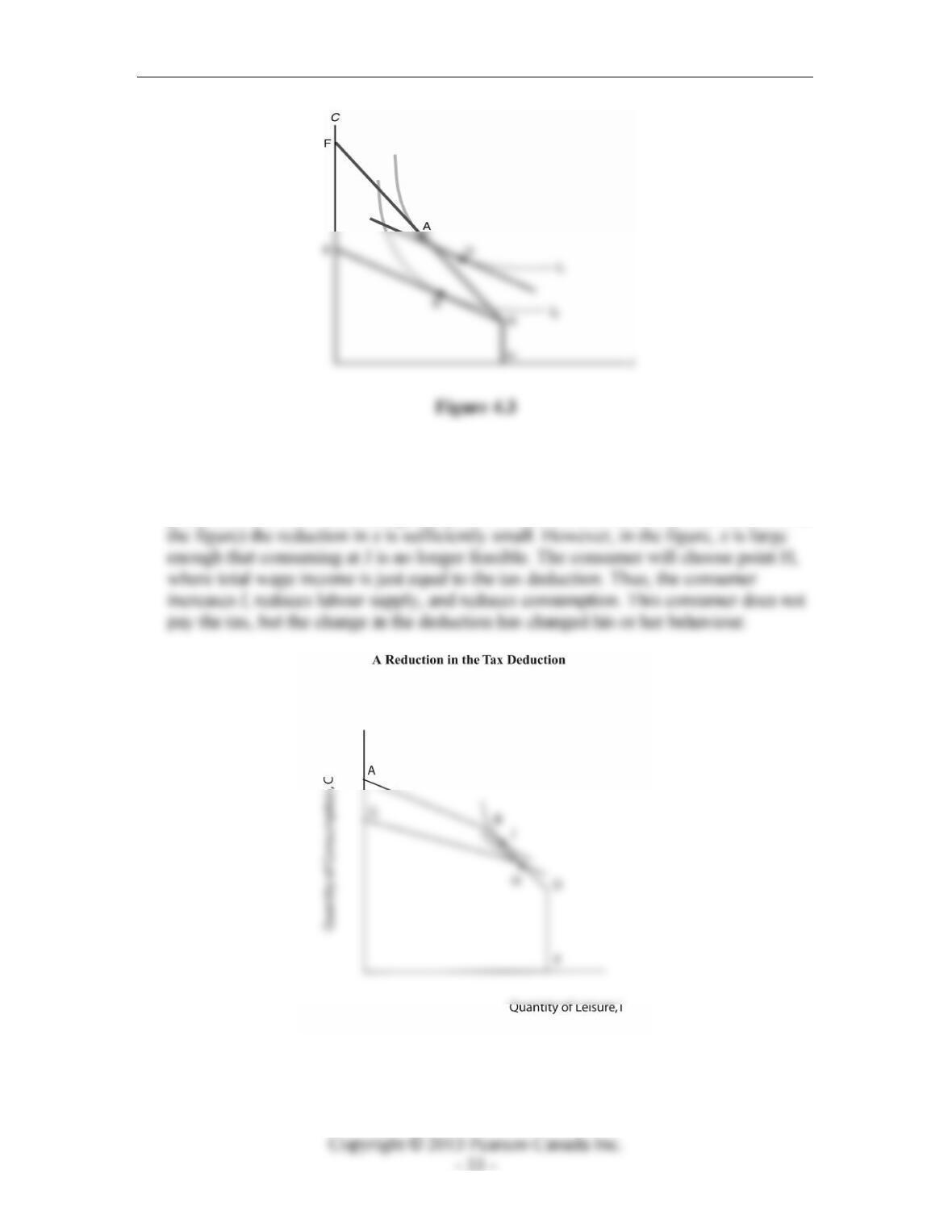
5. In Figure 4.4, the income tax deduction implies an extra kink in the budget constraint
of the consumer, so the initial budget constraint is ABDF. A reduction in the tax
deduction implies a shift in the budget constraint to GHDF. A consumer who chose a
point such as J before the change, may still choose J if (in contrast to what is shown in
Figure 4.4
Instructor’s Manual for Macroeconomics, Fourth Canadian Edition
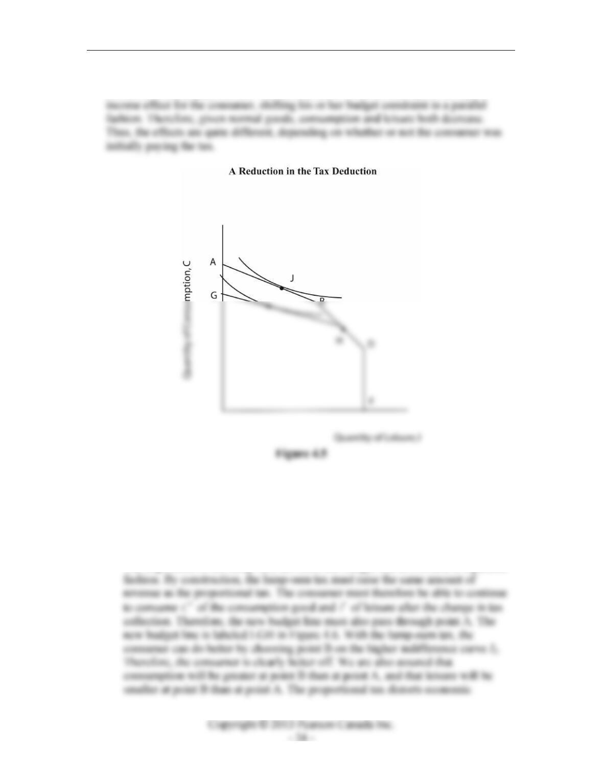
Now, suppose, as in Figure 4.5, that the consumer initially chooses point J, where the
consumer initially pays the tax. Then, a reduction in the tax deduction has a pure
6. Lump-Sum Tax versus Proportional Tax: Suppose that we start with a
proportional tax. Under the proportional tax the consumer’s budget line is EFH in
Figure 4.6. The consumer chooses consumption *
C and leisure *
l, at point A on
indifference curve I1. A shift to a lump-sum tax makes the budget line steeper.
The absolute value of the slope of the budget line is(1 )tw−and t has fallen to zero.
The imposition of the lump-sum tax shifts the budget line downward in a parallel

Chapter 4: Consumer and Firm Behaviour: The Work–Leisure Decision and Profit Maximization
7. The increase in dividend income shifts the budget line upward. The reduction in the
wage rate flattens the budget line. One possibility is depicted in Figure 4.7. The
original budget constraint HGL shifts to HFE. There are two income effects in this
Instructor’s Manual for Macroeconomics, Fourth Canadian Edition
Panel a Panel b
Panel c
Figure 4.7
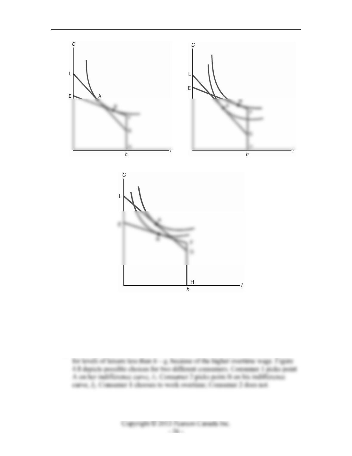
8. This problem introduces a higher overtime wage for hours worked above a threshold,
q. This problem also abstracts from any dividend income and taxes.
a) The budget constraint is now EJG in Figure 4.8. The budget constraint is steeper
Chapter 4: Consumer and Firm Behaviour: The Work–Leisure Decision and Profit Maximization
Figure 4.8
b) The geometry of Figure 4.8 makes it clear that it would be very difficult to have
c) An increase in the overtime wage makes the EJ segment of the budget constraint
steeper, but has no effect on the segment JG. For an individual like Consumer 2,
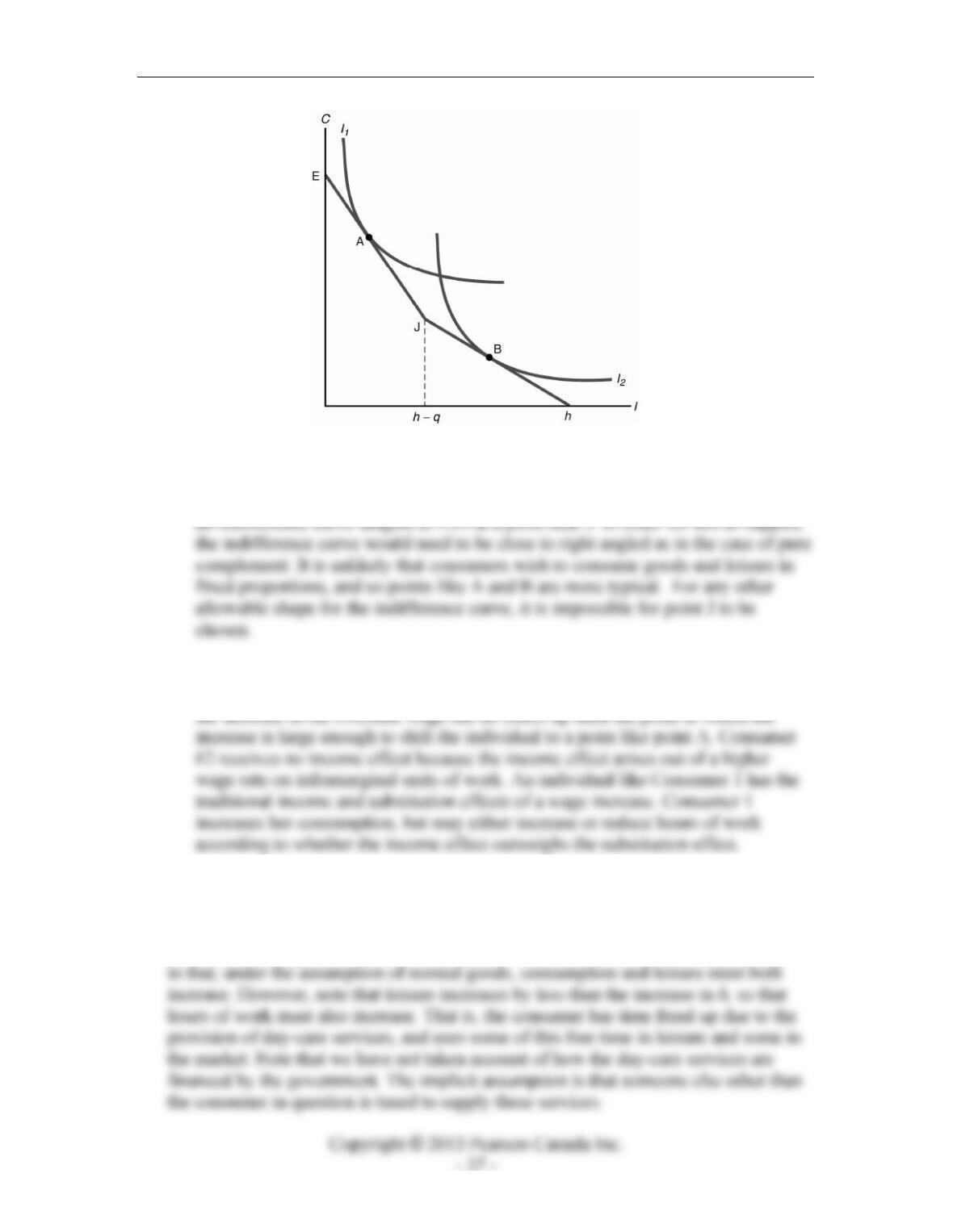
9. If h represents time not working in the market, then the provision of free day care
essentially increases h, as it reduces the amount of time spent in home production. In
Figure 4.9, this causes a parallel shift in the budget constraint of the consumer. The
effect on consumption and leisure works just as for an increase in non-wage income,
Instructor’s Manual for Macroeconomics, Fourth Canadian Edition
Provision of Day Care Services
Figure 4.9
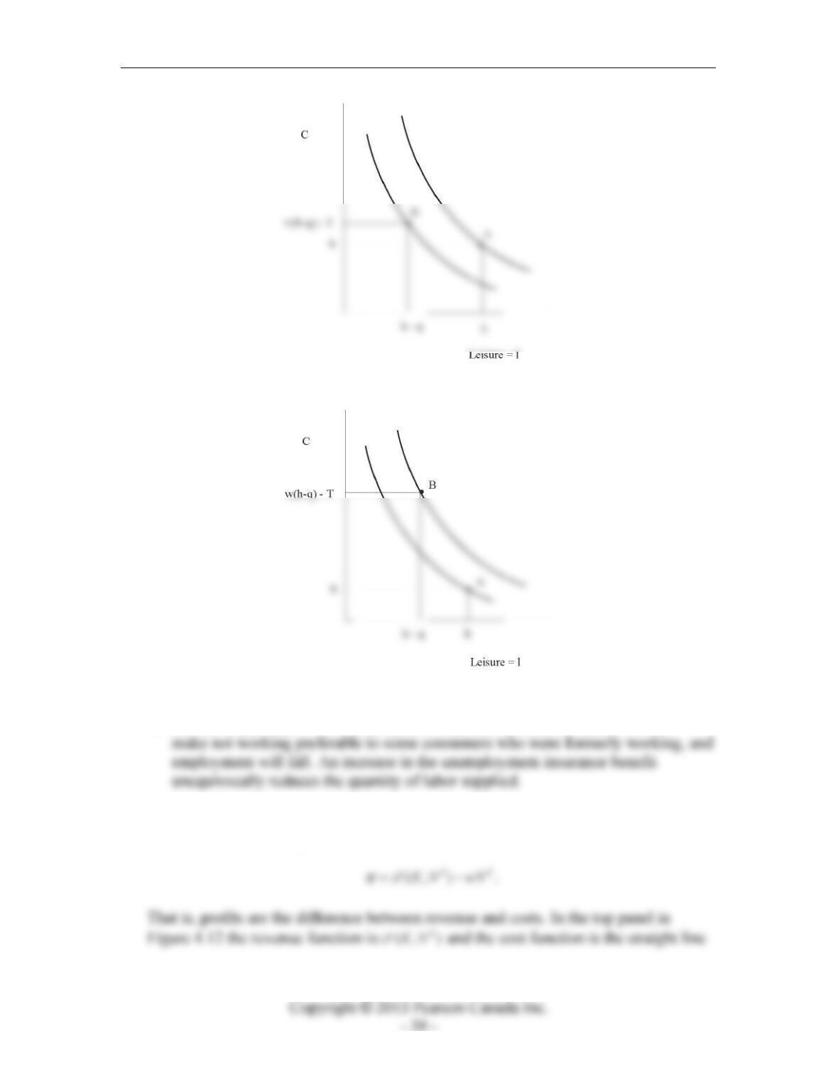
10. Supposing that the only options open to the consumer are working q hours and paying
a tax T, or working zero hours and receiving an unemployment insurance benefit b,
consumption will be w(h-q)-T if the consumer works, and b if the consumer decides
not to work. Then, either the consumer prefers not to work, as in the Figure 4.10,
where the highest indifference curve is achieved at point A rather than at point B, or
the consumer prefers to work, as in Figure 4.11. There is also another case where the
consumer is just indifferent between working and not working, but that case is not
important.
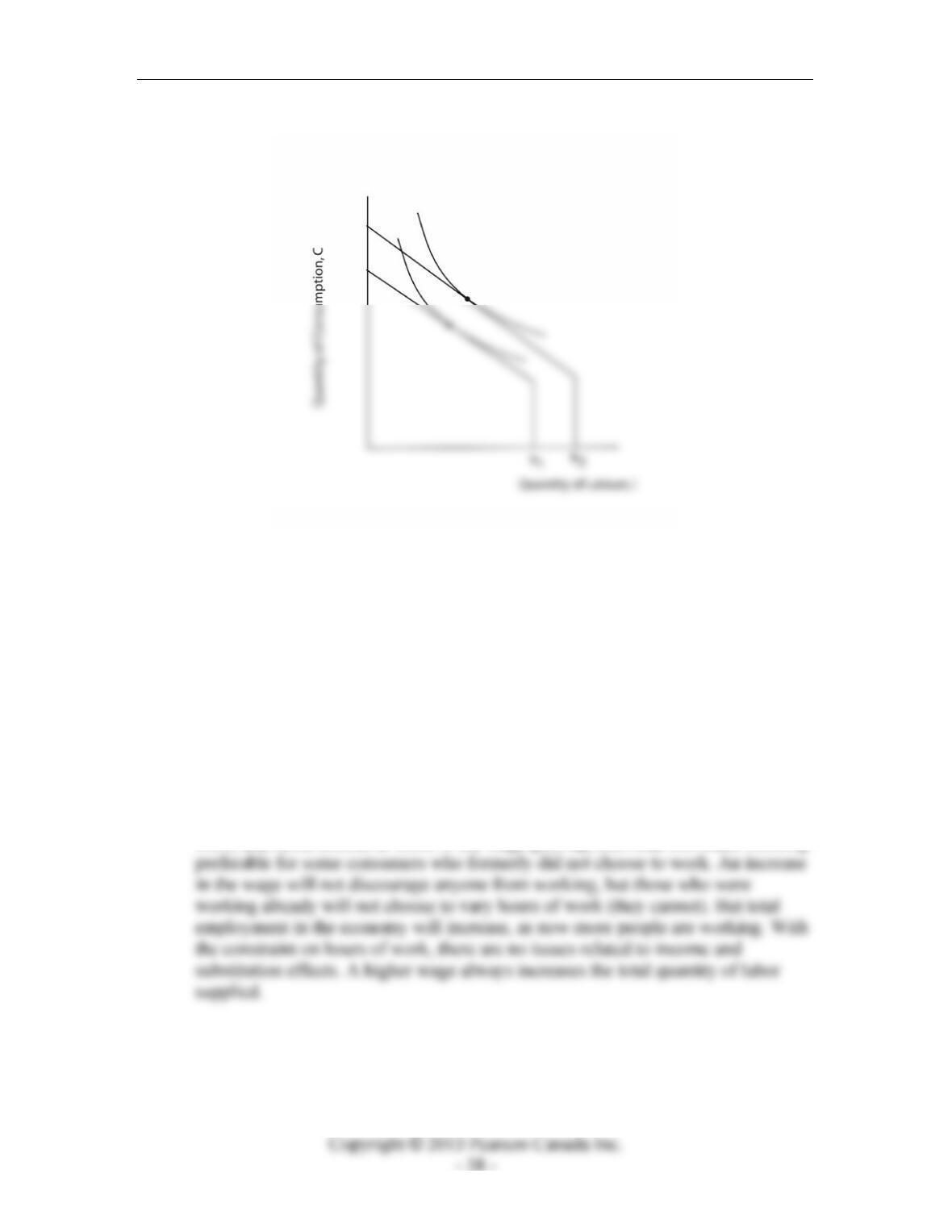
a) Think of the economy as consisting of many consumers, some of whom are in a
situation as in the Figure 4.10 and some as in Figure 4.11. Some consumers do not
work, and some choose to work. If the wage goes up, then that will make working
Chapter 4: Consumer and Firm Behaviour: The Work–Leisure Decision and Profit Maximization
Figure 4.10
Figure 4.11
b) Similar to part (a), if the unemployment insurance benefit increases, this will
11. The firm chooses its labour input, Nd, so as to maximize profits. When there is no tax,
profits for the firm are given by:
Instructor’s Manual for Macroeconomics, Fourth Canadian Edition
wNd. The firm maximizes profits by choosing the quantity of labour where the slope
of the revenue function equals the slope of the cost function:
With a tax that is proportional to the firm’s output, the firm’s profits are given by:
Here, the term (1 ) ( , )
d
tzFKN− is the after-tax revenue function and, as before, wNd is
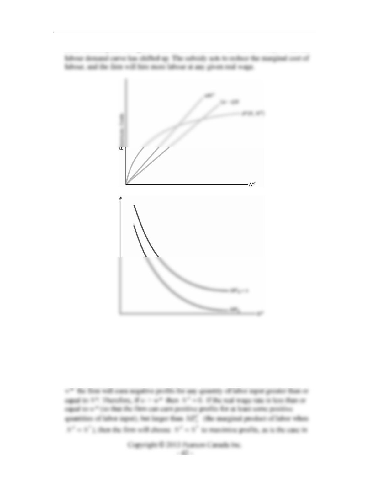
the cost function. In the top panel of Figure 4.12, the tax acts to shift down the
revenue function for the firm and reduces the slope of the revenue function. As
In the bottom panel of Figure 4.12, the labour demand curve is now(1 ) N
tMP− and the
labour demand curve has shifted down. The tax acts to reduce the after-tax marginal
product of labour, and the firm will hire less labour at any given real wage.
Chapter 4: Consumer and Firm Behaviour: The Work–Leisure Decision and Profit Maximization
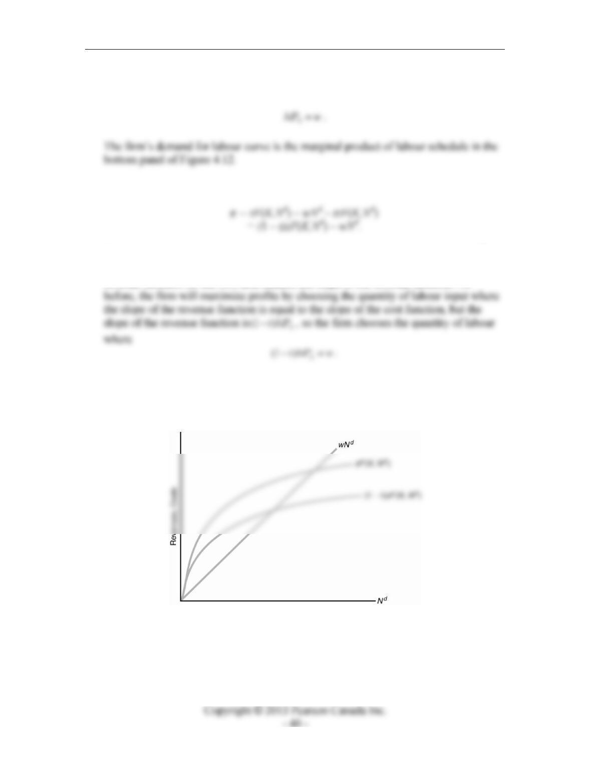
12. The firm chooses its labour input Nd so as to maximize profits. When there is no
subsidy, profits for the firm are given by
(, )
dd
zF K N wN
π
=−.
That is, profits are the difference between revenue and costs. In the top panel in
Figure 4.13 the revenue function is (, )
d
zF K N and the cost function is the straight line
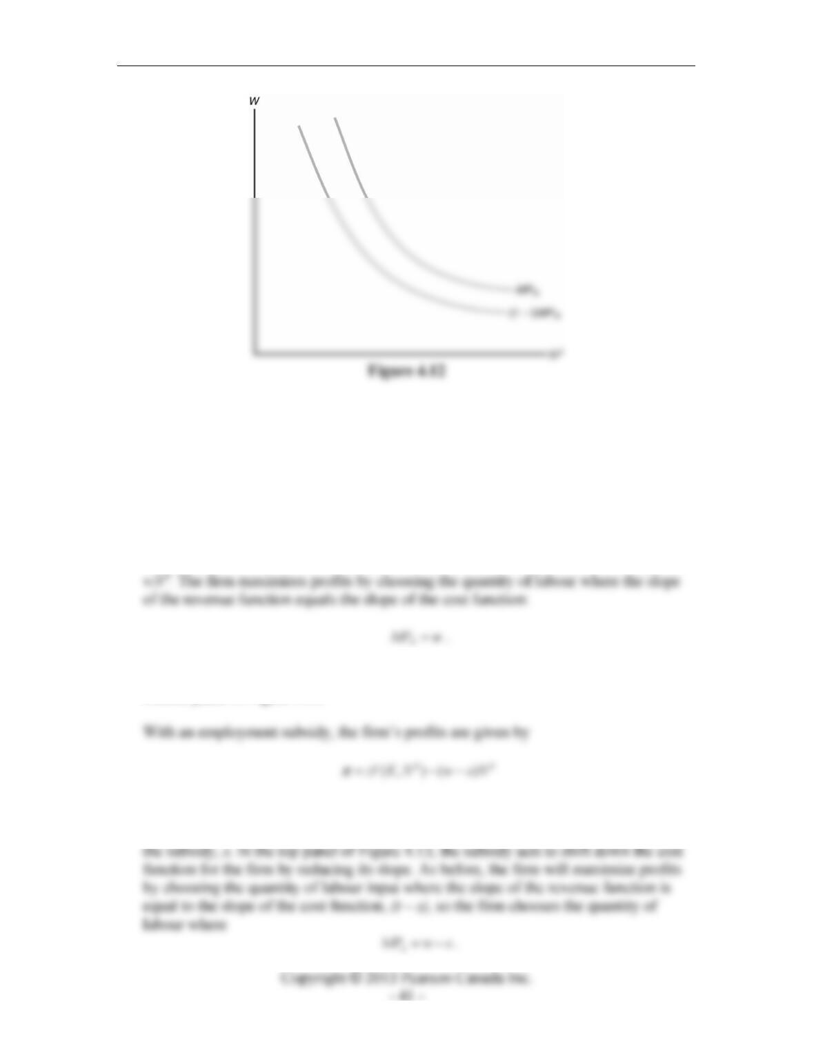
The firm’s demand for labour curve is the marginal product of labour schedule in the
bottom panel of Figure 4.13.
where, the term (, )
d
zF K N is the unchanged revenue function and (w – s)Nd is the cost
function. The subsidy acts to reduce the cost of each unit of labour by the amount of
Instructor’s Manual for Macroeconomics, Fourth Canadian Edition
In the bottom panel of Figure 4.13, the labour demand curve is now N
M
Ps+ and the
Figure 4.13
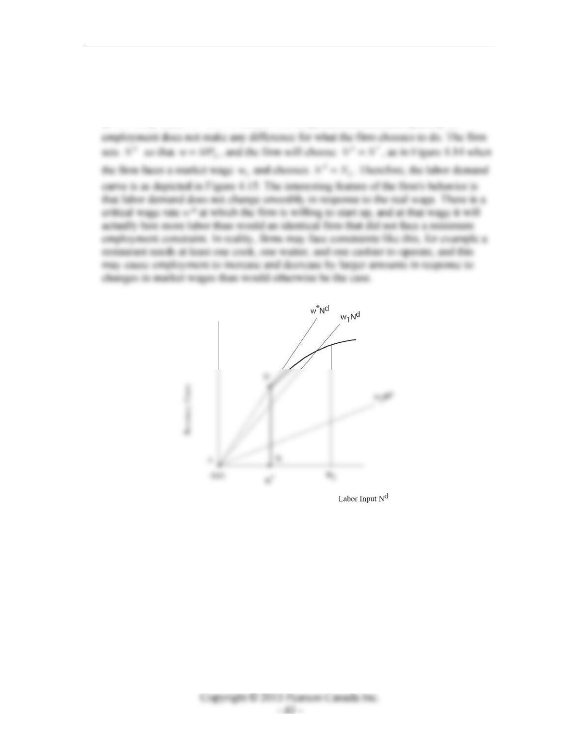
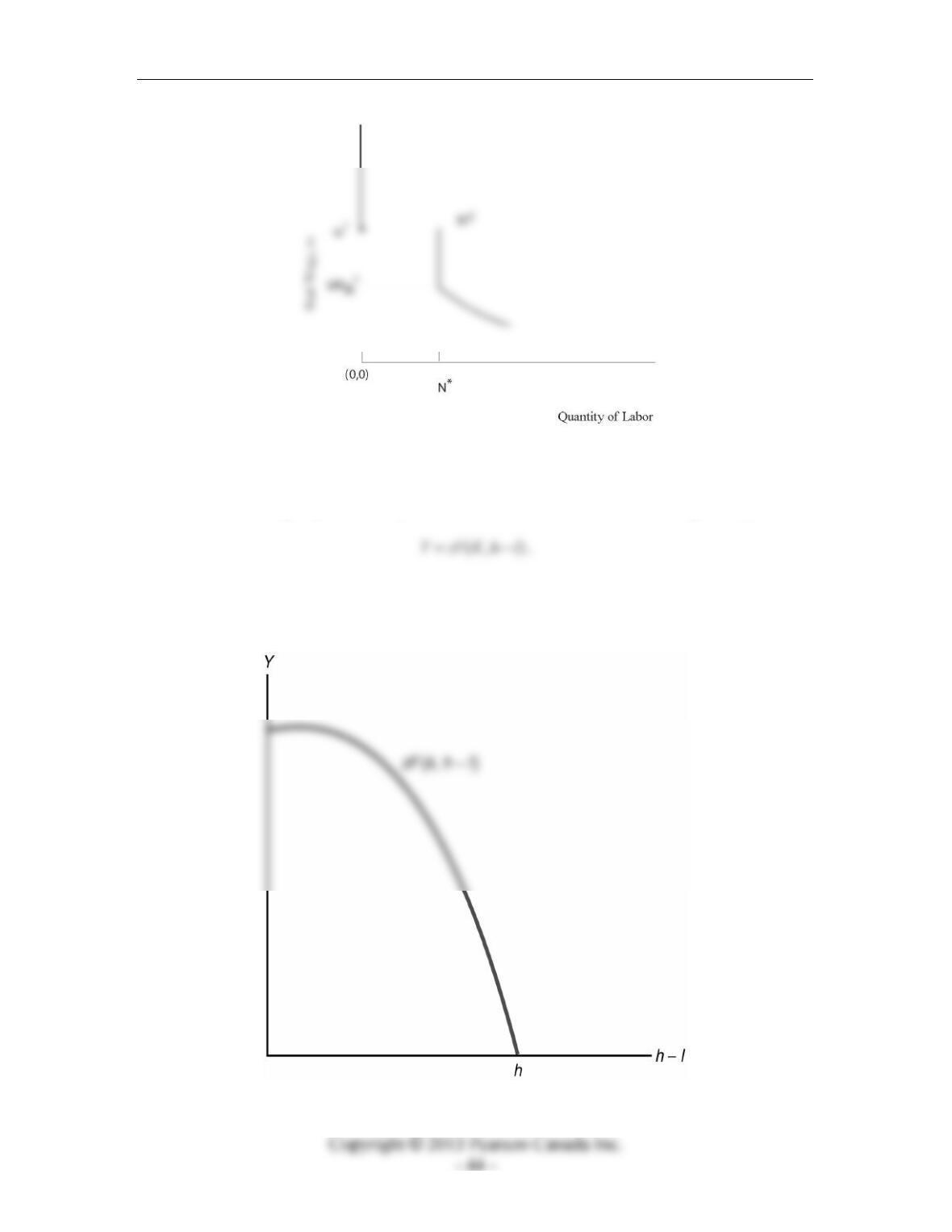
12. Minimum Employment Requirement: In Figure 4.14, given the minimum quantity
of employment that the firm requires to operate, the production function (indentical to
the total revenue function) follows ABD, and then continues along the same
production function we would have without the minimum quantity of employment.
The firm maximizes profits, which implies that, if the market wage rate is greater than
Chapter 4: Consumer and Firm Behaviour: The Work–Leisure Decision and Profit Maximization
Figure 4.14 when 1
ww=. That is, choosing *d
NN= is better than choosing 0
d
N=
in this case, because the firm will earn positive profits rather than zero profits.
However, if the firm increases the labor input above N*, this will just reduce profits,
as N
wMP> when *d
NN≥. Now, if *
wMP≤, then the minimum quantity of
Figure 4.14
Instructor’s Manual for Macroeconomics, Fourth Canadian Edition
Figure 4.15
14. The level of output produced by one worker who works h – l hours is given by:
This equation is plotted in Figure 4.16. The slope of this production possibilities
frontier is equal to N
M
P−.
Figure 4.16
15. The pollution regulation alters the firm’s profits according to
NxwY )1( +−=
π
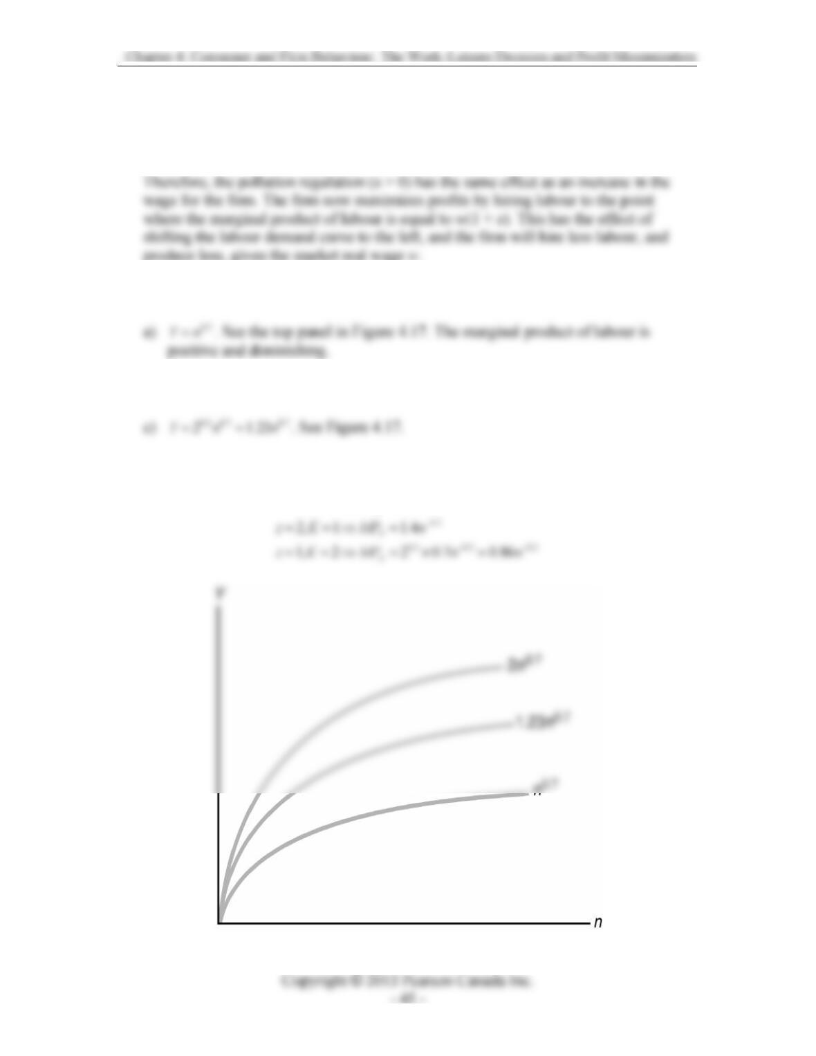
16. 0.3 0.7
YzKn=
b) 0.7
2Yn=. See Figure 4.17.
d) See the bottom panel of Figure 4.17.
0.3
1, 1 0.7
N
zK MP n
−
===
Instructor’s Manual for Macroeconomics, Fourth Canadian Edition
Figure 4.17
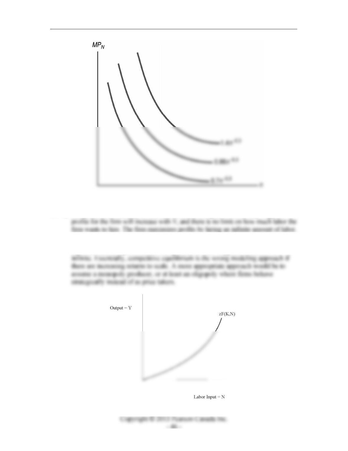
17. a) The production function, for fixed K, is shown in Figure 4.18. For any wage w,
b) This presents problems for competitive equilibrium because supply could never
equal demand in equilibrium, as the quantity of labor supplied could not be
Figure 4.18