Chapter 4
The Least Squares Estimator
◼ Exercises
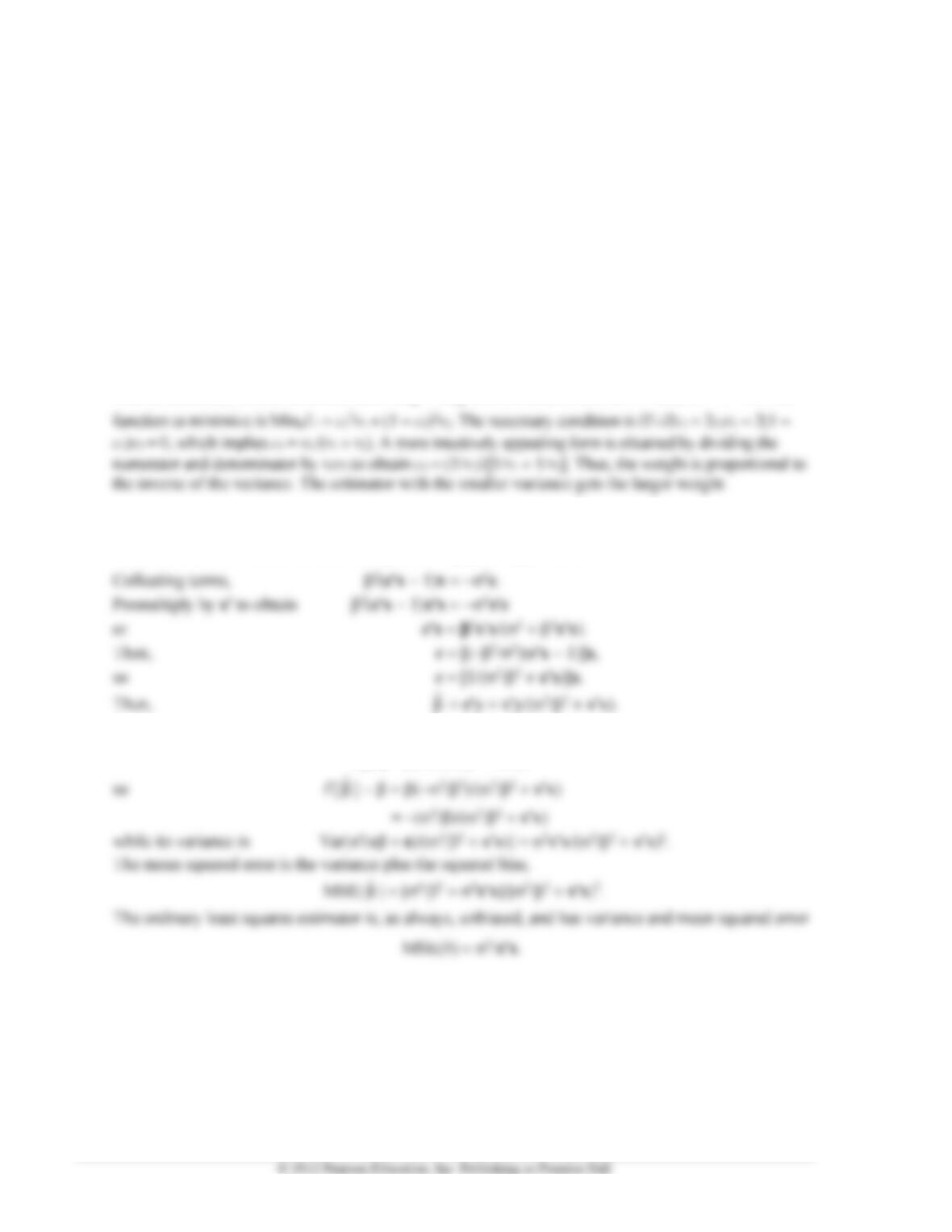
1. Consider the optimization problem of minimizing the variance of the weighted estimator. If the estimate
is to be unbiased, it must be of the form c1
1
ˆ
+ c2
2
ˆ
where c1 and c2 sum to 1. Thus, c2 = 1 − c1. The
2. First,
ˆ
= cy = cx + c. So, E[
ˆ
] = cx and Var[
ˆ
] = 2cc. Therefore, MSE[
ˆ
] = 2[cx − 1]2
+ 2cc. To minimize this, we set MSE[
ˆ
ˆ
]/c = 22[cx − 1]x + 22c = 0.
The expected value of this estimator is
E[
ˆ
ˆ
] = xx/(2/2 + xx)
Chapter 5 Hypothesis Tests and Model Selection 23
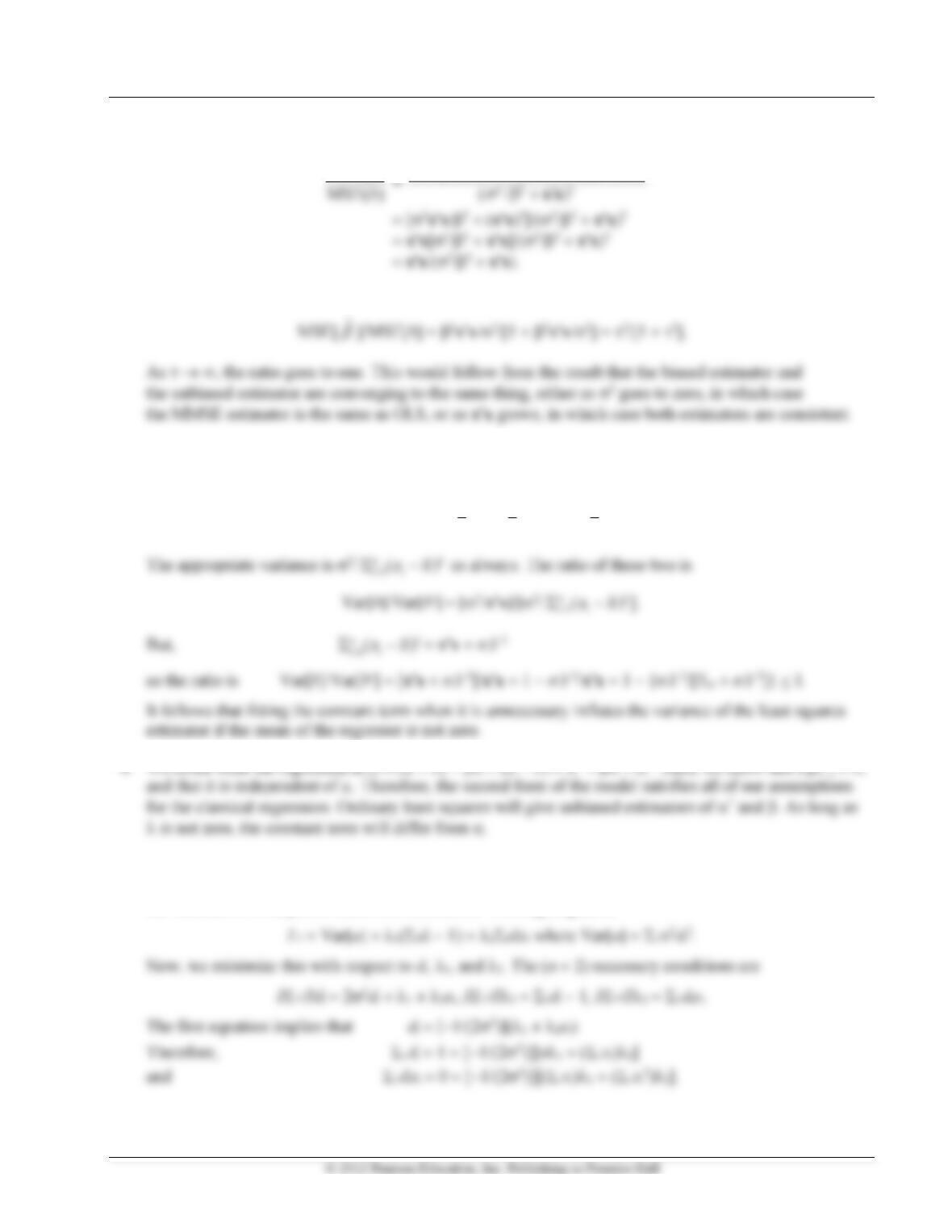
The ratio is taken by dividing each term in the numerator
ˆ
MSE[ ]
4 2 2 2 2
( / )/( / ) /( / )
+
x x x x x x
Now, multiply the numerator and denominator by 2/2 to obtain
3. The OLS estimator fit without a constant term is b = xy/xx. Assuming that the constant term is, in fact,
zero, the variance of this estimator is Var[b] = 2/xx. If a constant term is included in the regression,
then,
==
= − − − 2
11
( )( )/ ( ) .
nn
i i i i i
b x x y y x x
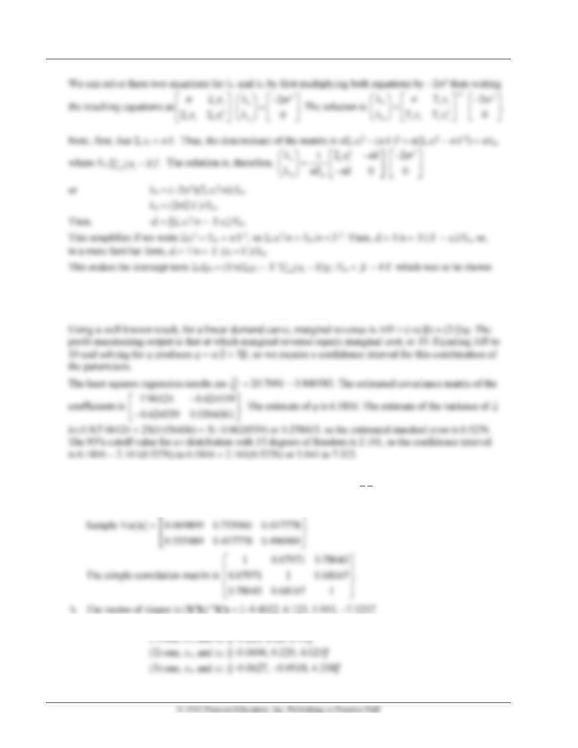
5. Let the constant term be written as a = idiyi = idi( + xi + i) = idi + idixi + idii. In order for a
to be unbiased for all samples of xi, we must have idi = 1 and idixi = 0. Consider, then, minimizing
the variance of a subject to these two constraints. The Lagrangean is
24 Greene • Econometric Analysis, Seventh Edition
6. Let q = E[Q]. Then,
q = + P, or P = (−/) + (1/)q.
7. a. The sample means are (1/100) times the elements in the first column of XX. The sample covariance
matrix for the three regressors is obtained as (1/99)[(XX) ij − 100
].
ij
xx
1.0127 0.069899 0.555489
c. For the three short regressions, the coefficient vectors are
Chapter 5 Hypothesis Tests and Model Selection 25
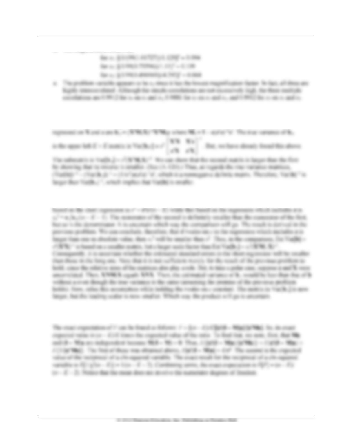
d. The magnification factors are
8. We consider two regressions. In the first, y is regressed on K variables, X. The variance of the least
squares estimator, b = (XX)−1Xy, Var[b] = 2(XX)−1. In the second, y is regressed on X and an
additional variable, z. Using results for the partitioned regression, the coefficients on X when y is
Although the true variance of b is smaller than the true variance of b.z, it does not follow that the estimated
variance will be. The estimated variances are based on s2, not the true 2. The residual variance estimator
9. The F-ratio is computed as [bXXb/K]/[ee/(n − K)]. We substitute e = M, and b = + (XX)−1X =
(XX)−1X. Then, F = [X(XX)−1XX(XX)−1X/K]/[M/(n − K)] = [(I − M)/K]/[M/(n − K)].
26 Greene • Econometric Analysis, Seventh Edition
10. We write b = + (XX)−1X, so bb = + X(XX)−1(XX)−1X + 2(XX)−1X. The expected value
of the last term is zero, and the first is nonstochastic. To find the expectation of the second term, use the
trace, and permute X inside the trace operator. Thus,
11. The F-ratio is computed as [bXXb/K]/[ee/(n − K)]. We substitute e = M, and b = + (XX)−1X =
13. The estimator is
y
= (1/n)i yi = (1/n)i ( + i) = + (1/n)i i. Then, E[
y
y
] = + (1/n)i E[i] = and
14. a. To solve this, we will use an extension of Exercise 5 in Chapter 3 (adding one row of data), and the
necessary matrix result, (A-66b) in which B will be Xm and C will be I. Bypassing the matrix algebra,
16. The coefficient vector is d = (ZZ)−1Zy. As assumed, Z = XCL, so d = (CL XXCL)−1 CL Xy. Also,
17. Using the results in Table 4.6 and the data given for the exercise,
matrix ; c = [-8.42653 / 1.33373 / -0.16537] $
28 Greene • Econometric Analysis, Seventh Edition
? Iterations, by trial and error.
calc ; delta = .005 $
First 3…
[CALC] LO = .3286204
[CALC] UO = 25.0149757
Calculator: Computed 5 scalar results
[CALC] LO = .0436204
Chapter 5 Hypothesis Tests and Model Selection 29
Applications
?=======================================================================
? Chapter 4 Application 1
?=======================================================================
Read $
Year GasExp Pop Gasp Income PNC PUC PPT PD PN PS
Sample ; 1 – 52 $
?=======================================================================
? a. Basic regression
?=======================================================================
Regress ; Lhs = g ; Rhs = X $
+—————————————————-+
| Ordinary least squares regression |
| LHS=G Mean = 4.935619 |
+—————————————————-+
+——–+————–+—————-+——–+——–+———-+
|Variable| Coefficient | Standard Error |t-ratio |P[|T|>t]| Mean of X|
+——–+————–+—————-+——–+——–+———-+
Constant| 1.10587817 .56937860 1.942 .0588
INCOME | .00021575 .517619D-04 4.168 .0001 16805.0577
?=======================================================================
? b. Hypothesis that b(NC) = b(UC) $
30 Greene • Econometric Analysis, Seventh Edition
?=======================================================================
? c. Elasticities. In each case, elasticity = b*xbar/ybar
?=======================================================================
Calc ; g2004 = g(52)$
Calc ; i2004 = income(52)$
+————————————+
| Listed Calculator Results |
+————————————+
EI = .948988
?=======================================================================
? d. Log regression
?=======================================================================
Create ; logg = log(g) ; logpg = log(gasp) ; logi = log(income)
+—————————————————-+
| Ordinary least squares regression |
| LHS=LOGG Mean = 1.570475 |
+—————————————————-+
+——–+————–+—————-+——–+——–+———-+
|Variable| Coefficient | Standard Error |t-ratio |P[|T|>t]| Mean of X|
+——–+————–+—————-+——–+——–+———-+
Constant| -7.28719016 2.52056245 -2.891 .0061
LOGI | .99299135 .25037574 3.966 .0003 9.67214751
Chapter 5 Hypothesis Tests and Model Selection 31
?=======================================================================
? e. Correlations of price variables
?=======================================================================
Namelist ; Prices = pnc,puc,ppt,pd,pn,ps$
Matrix ; list ; xcor(prices) $
Correlation Matrix for Listed Variables
PNC PUC PPT PD PN PS
PNC 1.00000 .99387 .98074 .99327 .98853 .97849
?=======================================================================
? f. Renormalizations of price variables
?=======================================================================
/*
In the linear case, the coefficients would be divided by the same
?=======================================================================
? g. Oaxaca decomposition
?=======================================================================
Dates ; 1953 $
Period ; 1953-1973 $
Matrix ; xb0 = Mean(logx)$
+————————————+
| Listed Calculator Results |
+————————————+
DYBAR = .395377
32 Greene • Econometric Analysis, Seventh Edition
?=======================================================================
? Chapter 4 Application 2
?=======================================================================
Create ; lc = log(cost/pf) ; lpl=log(pl/pf) ; lpk=log(pk/pf)$
? a. Cost function
Regress; lhs = lc ; rhs = x ; printvc $
+—————————————————-+
| Ordinary least squares regression |
| LHS=LC Mean = -.3195570 |
+—————————————————-+
+——–+————–+—————-+——–+——–+———-+
|Variable| Coefficient | Standard Error |t-ratio |P[|T|>t]| Mean of X|
+——–+————–+—————-+——–+——–+———-+
Constant| -6.81816332 .25243920 -27.009 .0000
1 2 3 4 5
+———————————————————————-
1| .06373 -.00238 .00031 .00399 -.01047
?=======================================================================
? b. Capital price coefficient
?=======================================================================
Wald ; fn1 = 1 – b_lpk – b_lpl $
+———————————————–+
| WALD procedure. Estimates and standard errors |
| for nonlinear functions and joint test of |
| nonlinear restrictions. |
+———————————————–+
+——–+————–+—————-+——–+——–+
|Variable| Coefficient | Standard Error |b/St.Er.|P[|Z|>z]|
Chapter 5 Hypothesis Tests and Model Selection 33
?=======================================================================
? c. Efficient scale
?=======================================================================
Wald ; fn1 = exp((1-b_lq)/b_lqq) $
+———————————————–+
| WALD procedure. Estimates and standard errors |
| for nonlinear functions and joint test of |
| nonlinear restrictions. |
+——–+————–+—————-+——–+——–+
|Variable| Coefficient | Standard Error |b/St.Er.|P[|Z|>z]|
?=======================================================================
? d. Raw data
?=======================================================================
+————————————+
| Listed Calculator Results |
+————————————+