Chapter 4
Consumption, Saving, and Investment
◼ Learning Objectives
I. Goals of Chapter 4
A. Describe the factors that affect consumption and saving decisions (Sec. 4.1)
II. Notes to Eighth Edition Users
A. We changed the term “expected after–tax real interest rate” to “expected real after-tax interest
64 Abel/Bernanke/Croushore • Macroeconomics, Ninth Edition
◼ Teaching Notes
I. Consumption and Saving (Sec. 4.1)
A. The importance of consumption and saving
Data Application
Recall from Chapter 2 that measured consumption in the national income accounts includes
spending on durable consumption goods, like autos and major appliances. But consumption
B. The consumption and saving decision of an individual
1. A person can consume less than current income (saving is positive)
C. Effect of changes in current income
1. Increase in current income: both consumption and saving increase (vice versa for decrease in
current income)
Theoretical Application
The classic discussions of consumption are the permanent-income hypothesis of Milton
Friedman (A Theory of the Consumption Function, Princeton: Princeton University Press, 1957)
D. Effect of changes in expected future income
1. Higher expected future income leads to more consumption today, so saving falls

Chapter 4 Consumption, Saving, and Investment 65
2. Application: consumer sentiment and forecasts of consumer spending
a. Do consumer sentiment indexes help economists forecast consumer spending?
E. Effect of changes in wealth
1. Increase in wealth raises current consumption, so lowers current saving
F. Effect of changes in real interest rate
1. Increased real interest rate has two opposing effects
a. Substitution effect: Positive effect on saving, since rate of return is higher; greater reward
Theoretical Application
You can use the concept of income and substitution effects to show your class how saving responds
to an effective change in the expected real interest rate that occurs because of IRAs (individual
retirement accounts). Since IRAs allow people to avoid taxes on a portion of their income, they
saving rises or falls depends on whether, in the absence of IRAs, they would have saved more or less.
Empirical evidence suggests that every $100 of IRA saving reduces current consumption by $32, so
at least for some people, the substitution effect is strong enough to increase saving.
2. Taxes and the real return to saving
a. Expected real after-tax interest rate:

3. In touch with data and research: interest rates
a. Discusses different interest rates, default risk, term structure (yield curve), and tax status
G. Fiscal policy
1. Affects desired consumption through changes in current and expected future income
2. Directly affects desired national saving, Sd = Y − Cd − G
3. Government purchases (temporary increase)
a. Higher G financed by higher current taxes reduces after-tax income, lowering desired
consumption
Data Application
This theory is confirmed by empirical data. Shaghil Ahmed, in “Temporary and Permanent
4. Taxes
a. Lump-sum tax cut today, financed by higher future taxes

Chapter 4 Consumption, Saving, and Investment 67
tax cut leads to increased desired consumption and reduced desired national saving
Theoretical Application
There are a number of reasons why Ricardian equivalence may not hold. The text notes that if
people don’t see that future taxes are equal (in present value) to a current tax cut, then Ricardian
equivalence may not hold. An additional reason for the failure of Ricardian equivalence,
liquidity constraints, is covered in Appendix 4.A. It may also be possible for people to avoid
H. Application: How consumers respond to tax rebates
1. The government provided tax rebates in the recessions of 2001 and 2007–2009, hoping to
stimulate the economy
2. Research by Shapiro and Slemrod suggests that consumers did not increase spending much
II. Investment (Sec. 4.2)
A. Why is investment important?
1. Investment fluctuates sharply over the business cycle, so we need to understand investment
to understand the business cycle
2. Investment plays a crucial role in economic growth
68 Abel/Bernanke/Croushore • Macroeconomics, Ninth Edition
B. The desired capital stock
1. Desired capital stock is the amount of capital that allows firms to earn the largest expected profit
2. Desired capital stock depends on costs and benefits of additional capital
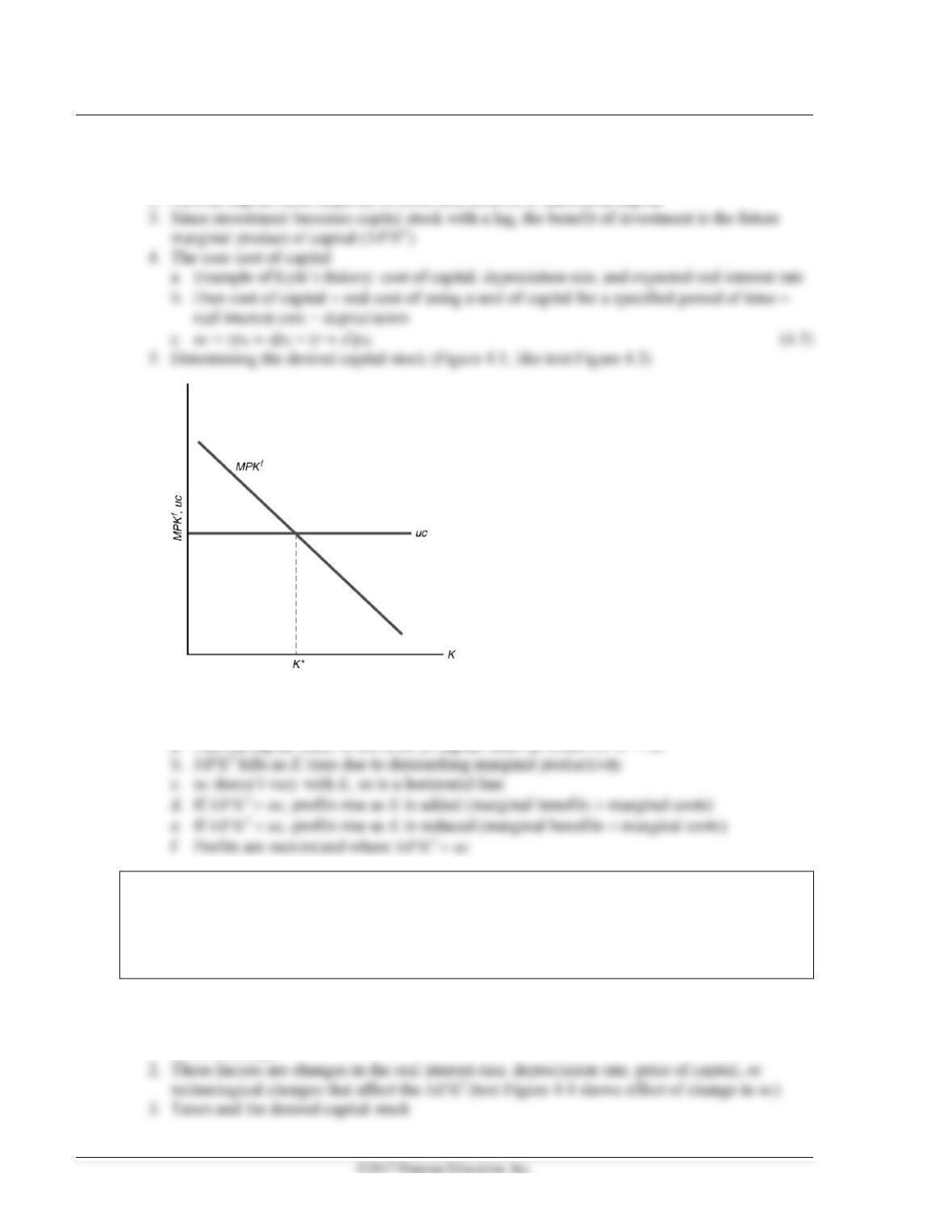
Figure 4.1
a. Desired capital stock is the level of capital stock at which MPKf = uc
Theoretical Application
The first general use of the user cost of capital concept was by Dale Jorgenson, “Capital Theory
and Investment Behavior,” American Economic Review Papers and Proceedings, May 1963,
pp. 247–259.
C. Changes in the desired capital stock
1. Factors that shift the MPKf curve or change the user cost of capital cause the desired capital
stock to change
Chapter 4 Consumption, Saving, and Investment 69
a. With taxes, the return to capital is only (1 −
)MPKf
Numerical Problems 2 and 4 give students practice in working with the marginal product of
capital and the user cost of capital.
e. In reality, there are complications to the tax-adjusted user cost
(1) We assumed that firm revenues were taxed
(2) Investment tax credits reduce taxes when firms make new investments
(3) Summary measure: the effective tax rate—the tax rate on firm revenue that would
Data Application
Another simplification that is used in this chapter is the assumption that taxes are based on a
f. Application: measuring the effects of taxes on investment
(1) Do changes in the tax rate have a significant effect on investment?
Theoretical Application
For further discussions of the effects of tax policy on investment, see Robert E. Hall and Dale W.
Jorgenson, “Tax Policy and Investment Behavior,” American Economic Review, June 1967,
pp. 391–414.
D. From the desired capital stock to investment
1. The capital stock changes from two opposing channels
a. New capital increases the capital stock; this is gross investment

70 Abel/Bernanke/Croushore • Macroeconomics, Ninth Edition
2. Rewriting (4.5) gives It = Kt+1 − Kt + dKt
a. If firms can change their capital stocks in one period, then the desired capital stock
(K*) = Kt+1
a. Some capital can be constructed easily, but other capital may take years to put in place
Theoretical Application
Acknowledging that it may take time to get capital in place may be crucial to modeling the
Fluctuations,” Econometrica, November 1982, pp. 1345–1370.
b. So investment needed to reach the desired capital stock may be spread out over several
years
E. In touch with data and research: investment and the stock market
2. If market value replacement cost, then firm should invest more
3. Tobin’s q = capital’s market value divided by its replacement cost
4. Stock price times number of shares equals firm’s market value, which equals value
of firm’s capital
5. Data show general tendency of investment to rise when stock market rises; but relationship
isn’t strong because many other things change at same time (text Fig. 4.7)
F. Investment in inventories and housing
1. Marginal product of capital and user cost also apply, as with equipment and structures
Numerical Problem 3 applies the user-cost concept to the purchase or rental of a home.
III. Goods Market Equilibrium (Sec. 4.3)

Chapter 4 Consumption, Saving, and Investment 71
A. The real interest rate adjusts to bring the goods market into equilibrium
1. Y = Cd + Id + G (4.7)
Sd = Id (4.8)
B. The saving-investment diagram
1. Plot Sd vs. Id (Figure 4.2; Key Diagram 3; like text Figure 4.8)
2. Equilibrium where Sd = Id
3. How to reach equilibrium? Adjustment of r
4. Shifts of the saving curve
a. Saving curve shifts right due to a rise in current output, a fall in expected future output,
Numerical Problem 5 and 6 and Analytical Problem 5 examine what happens when government
spending changes.
Theoretical Application
What happens to the economy if government taxes change? Under Ricardian equivalence, a tax cut

72 Abel/Bernanke/Croushore • Macroeconomics, Ninth Edition
5. Shifts of the investment curve
a. Investment curve shifts right due to a fall in the effective tax rate or a rise in expected
C. Application: Macroeconomic consequences of the boom and bust in stock prices
1. Sharp changes in stock prices affect consumption spending (a wealth effect) and capital
investment (via Tobin’s q), seen in text Figure 4.11
2. Consumption and the 1987 crash
a. When the stock market crashed in 1987, wealth declined by about $1 trillion
3. Consumption and the rise in stock market wealth in the 1990s
4. Consumption and the decline in stock prices in the early 2000s
5. Investment and the declines in the stock market in the 2000s
a. Investment and Tobin’s q were correlated in 2000 and 2008, when the stock market fell
6. The financial crisis of 2008
a. Stock prices plunged in fall 2008 and early 2009, and home prices fell sharply as well,
leading to a large decline in household net wealth
b. Despite the decline in wealth, the ratio of consumption to GDP did not decline much
Policy Application
Should tax policy be used to promote savings or investment? Many policymakers and
economists have argued that obtaining the correct amount of future economic growth requires us
Chapter 4 Consumption, Saving, and Investment 73
Analytical Problems 1, 2, 3, and 4 all look at shocks to the economy and changes in variables
needed to restore equilibrium.
IV. Appendix 4.A: A Formal Model of Consumption and Saving
A. How much can the consumer afford? The budget constraint
1. Current income y; future income yf; initial wealth a
B. The budget line
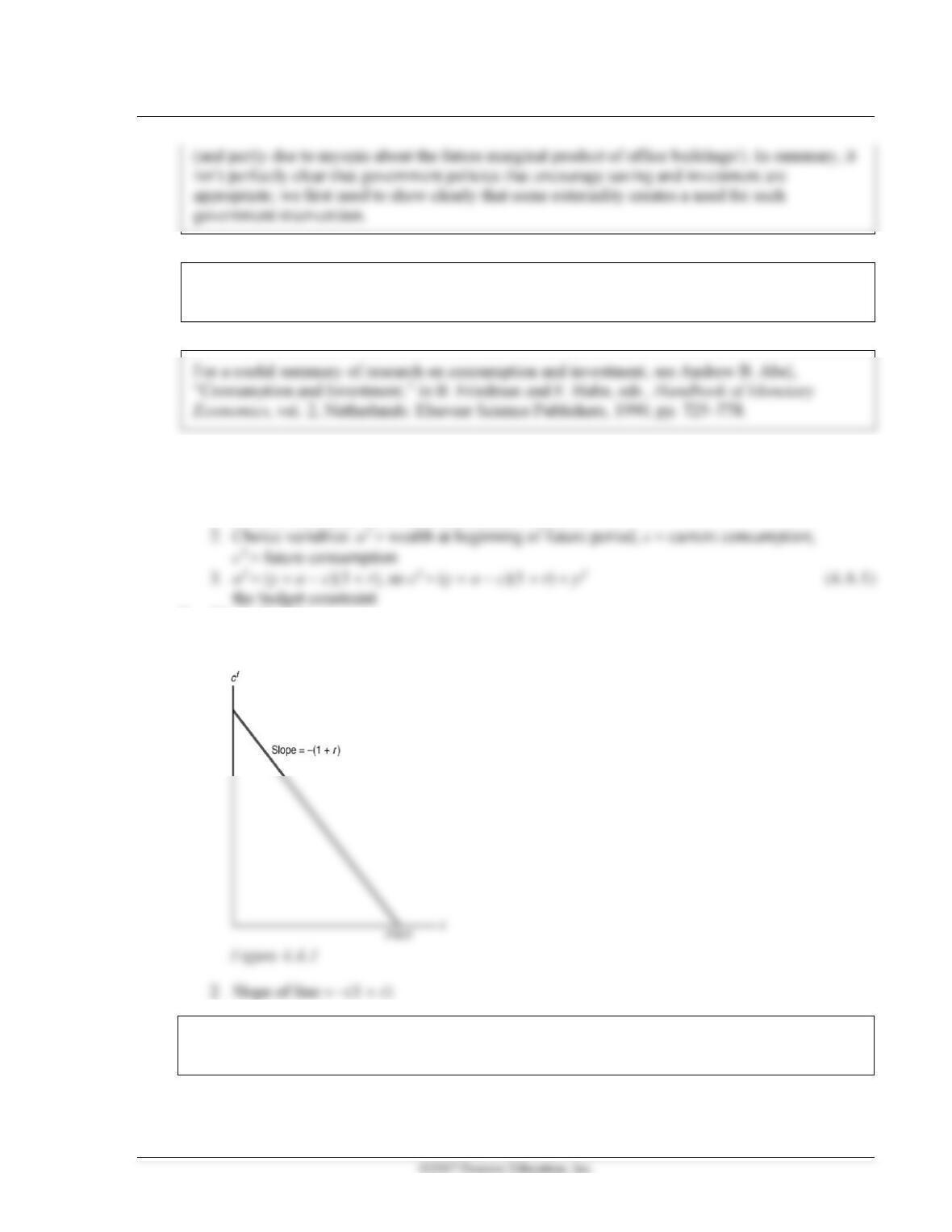
1. Graph budget line in (c, cf) space (Figure 4.A.1)
Analytical Problem 7 looks at what happens to the budget line when the interest rate on
borrowing differs from the interest rate on lending.
C. Present values

74 Abel/Bernanke/Croushore • Macroeconomics, Ninth Edition
1. Present value is the value of payments to be made in the future in terms of today’s dollars or
goods
Chapter 4 Consumption, Saving, and Investment 75
Once you’ve established the intuition about the present value formula for one period, you can
D. Present value and the budget constraint
1. Present value of lifetime resources:
PVLR = y + yf/(1 + r) + a (4.A.2)
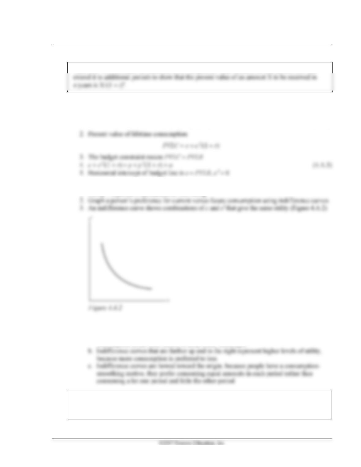
E. What does the consumer want? Consumer preferences
1. Utility = a person’s satisfaction or well-being
4. A person is equally happy at any point on an indifference curve
5. Three important properties of indifference curves
a. Slope downward from left to right: Less consumption in one period requires more
consumption in the other period to keep utility unchanged
If students want more help on indifference curves, you can refer them to a principles of economics
or intermediate microeconomics text, such as Michael Parkin, Economics, 5th edition, Reading,
Mass.: Addison Wesley Longman, 2000.
76 Abel/Bernanke/Croushore • Macroeconomics, Ninth Edition
F. The optimal level of consumption
1. Optimal consumption point is where the budget line is tangent to an indifference curve
(Figure 4.A.3)
2. That’s the highest indifference curve that it’s possible to reach
3. All other points on the budget line are on lower indifference curves
G. The Effects of Changes in Income and Wealth on Consumption and Saving
1. The effect on consumption of a change in income (current or future) or wealth depends
only on how the change affects the PVLR
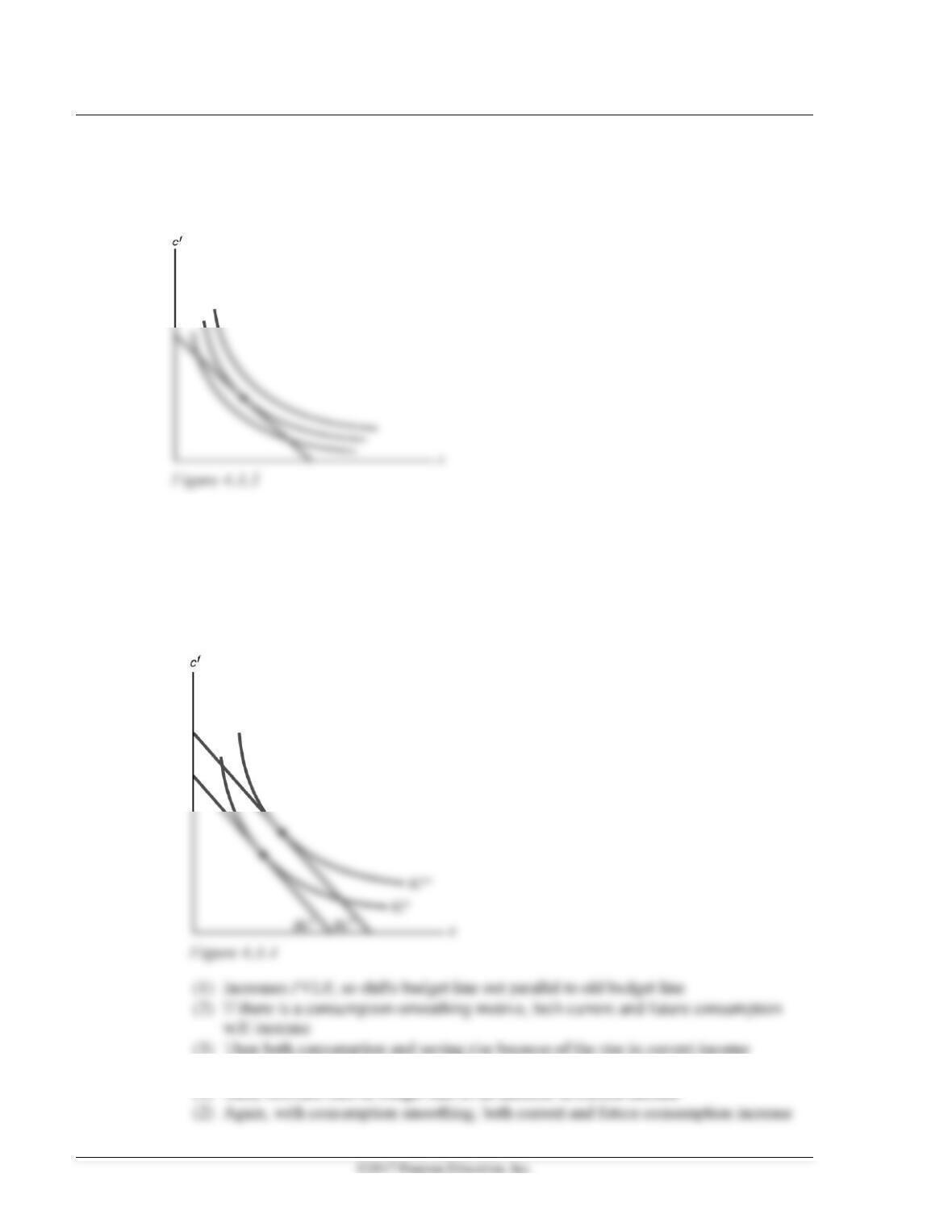
a. An increase in current income (Figure 4.A.4)
(3) Then both consumption and saving rise because of the rise in current income
b. An increase in future income
(1) Same outward shift in budget line as an increase in current income

Chapter 4 Consumption, Saving, and Investment 77
c. An increase in wealth
(1) Same parallel shift in budget line, so both current and future consumption rise
Numerical Problem 8 deals with the income effect on consumption and saving.
d. The permanent income theory
(1) Different types of changes in income
(2) Permanent income increase causes bigger increase in PVLR than a temporary income
increase
(3) This distinction between permanent and temporary income changes was made by
Milton Friedman in the 1950s and is known as the permanent income theory
H. Consumption and Saving Over Many Periods: The Life-Cycle Model
1. Life-cycle model was developed by Franco Modigliani and associates in the 1950s
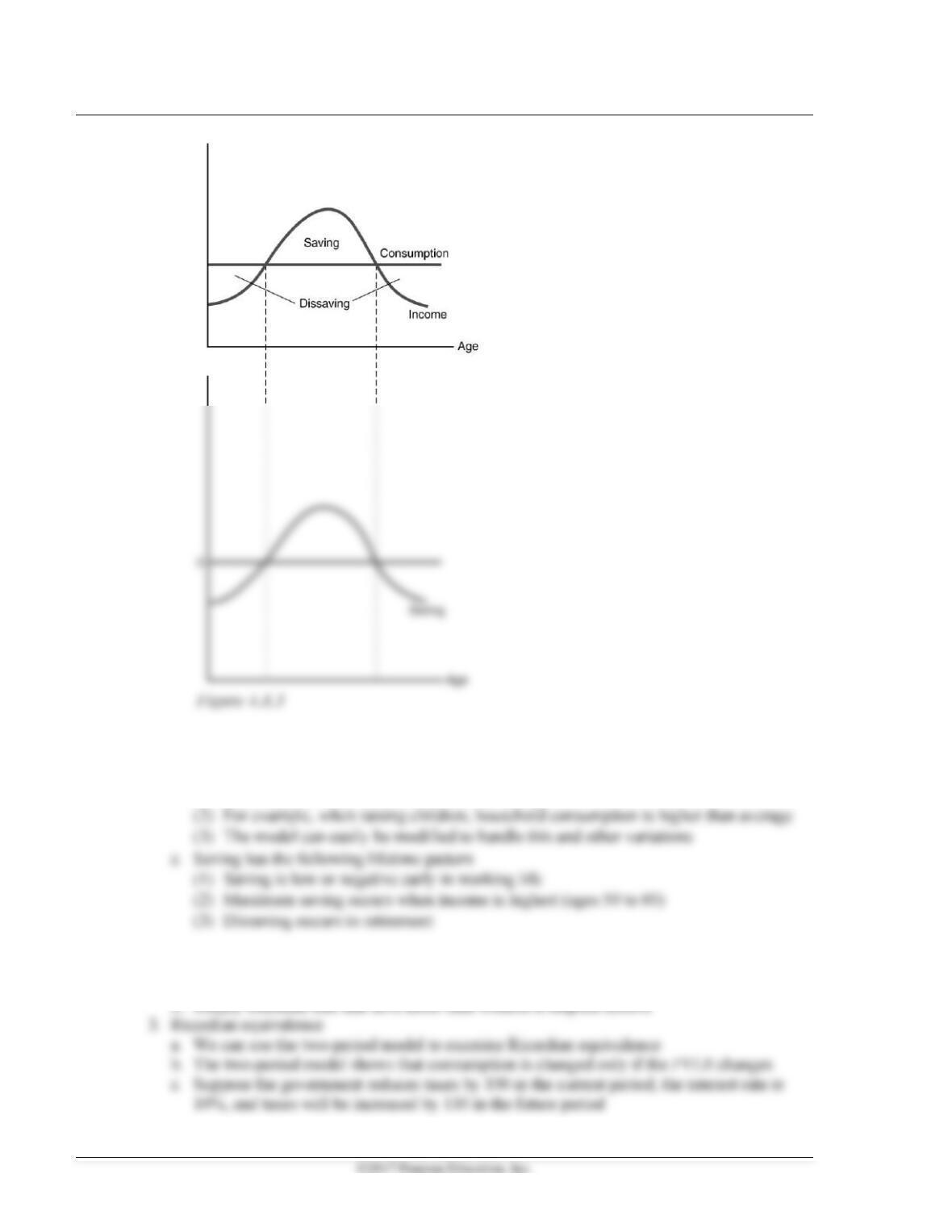
a. Looks at patterns of income, consumption, and saving over an individual’s lifetime
78 Abel/Bernanke/Croushore • Macroeconomics, Ninth Edition
c. Real income steadily rises over time until near retirement; at retirement, income drops
sharply
d. Lifetime pattern of consumption is much smoother than the income pattern
(1) In reality, consumption varies somewhat by age
2. Bequests and saving
a. What effect does a bequest motive (a desire to leave an inheritance) have on saving?
Chapter 4 Consumption, Saving, and Investment 79
d. Then the PVLR is unchanged, and thus there is no change in consumption
4. Excess sensitivity and borrowing constraints
a. Generally, theories about consumption, including the permanent income theory, have
(1) This could be due to shortsighted behavior
(2) Or it could be due to borrowing constraints
d. Borrowing constraints mean people can’t borrow as much as they want Lenders may
worry that a consumer won’t pay back the loan, so they won’t lend
Numerical Problem 9 deals with borrowing constraints.
I. The Real Interest Rate and the Consumption-Saving Decision
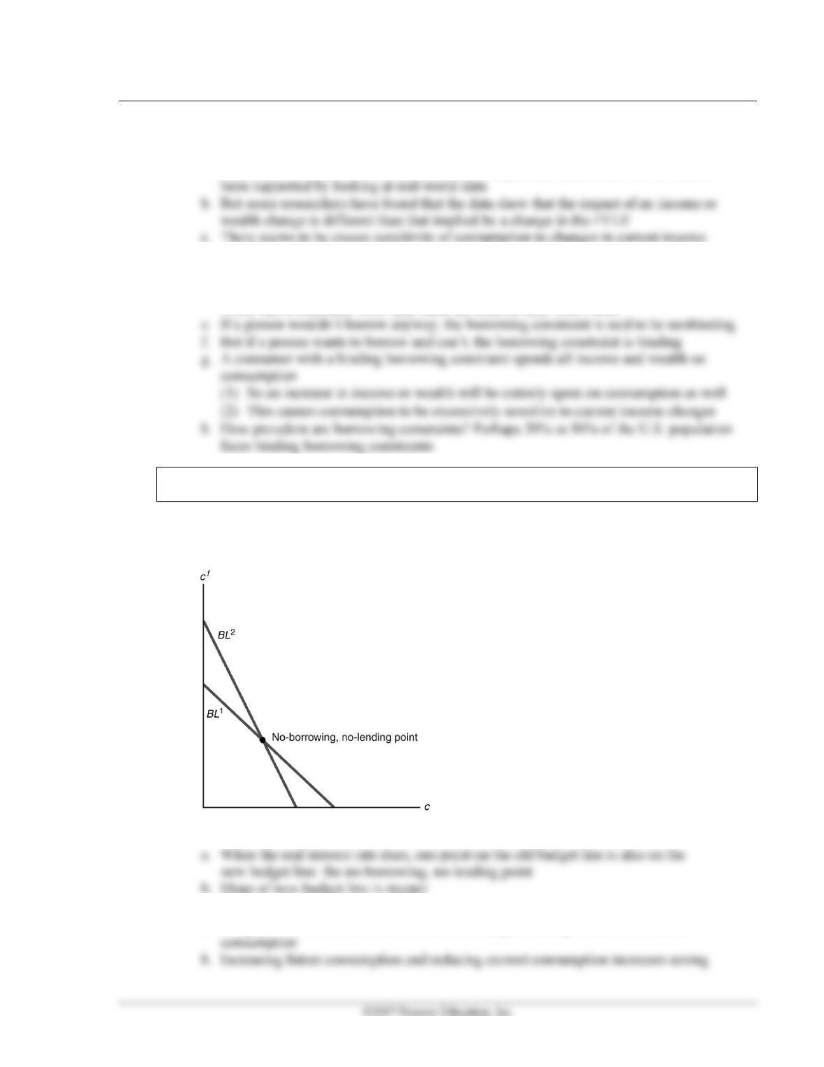
1. The real interest rate and the budget line (Figure 4.A.6)
Figure 4.A.6
2. The substitution effect
a. A higher real interest rate makes future consumption cheaper relative to current
80 Abel/Bernanke/Croushore • Macroeconomics, Ninth Edition
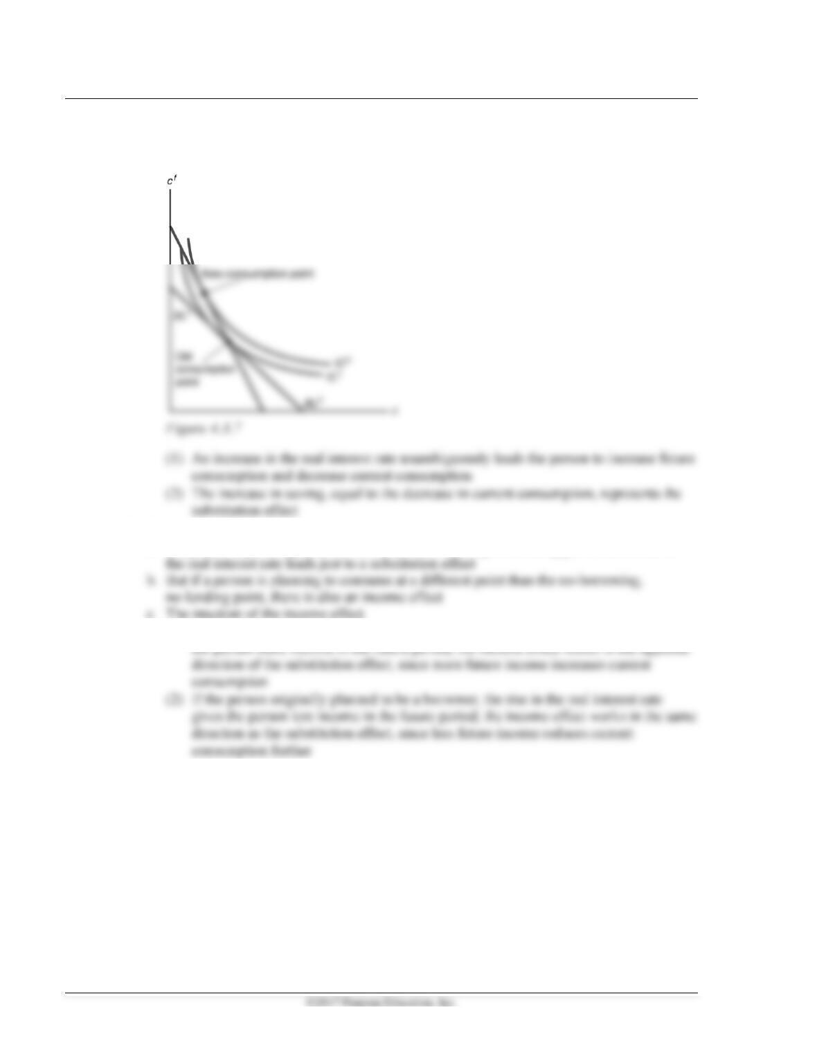
c. Suppose a person is at the no-borrowing, no-lending point when the real interest rate rises
(Figure 4.A.7)
3. The income effect
a. If a person is planning to consume at the no-borrowing, no-lending point, then a rise in
(1) If the person originally planned to be a lender, the rise in the real interest rate gives

4. The income and substitution effects together
a. Split the change in the budget line into two parts (Figure 4.A.8)
(1) A budget line with the same slope as the new budget line, but going through the
original consumption point (BLint)
(2) The substitution effect is shown by the change from budget line BL1 to budget line
Analytical Problem 6 asks the student to show the income and substitution effects for a borrower.
e. The effect on aggregate saving of a rise in the real interest rate is ambiguous theoretically