Demand and Supply 63
B. During the summer month of July, the variable S = 1. Therefore, assuming that price-
related values remain as before, the firm demand curve is:
P3.7 Supply Function. A review of industry wide data for the jelly and jam manufacturing
industry suggests the following industry supply function:
Q = -59,000,000 + 500,000P – 125,000PL
– 500,000PK + 2,000,000W,
where Q is cases supplied per year, P is the wholesale price per case ($), PL is the
average price paid for unskilled labor ($), PK is the average price of capital (in percent),
and W is weather measured by the average seasonal rainfall in growing areas (in
inches).
A. Determine the industry supply curve for a recent year when PL = $8, PK = 10
C. Calculate the prices necessary to generate a supply of 4 million, 6 million, and 8
million cases.
64 Chapter 3
P3.7 SOLUTION
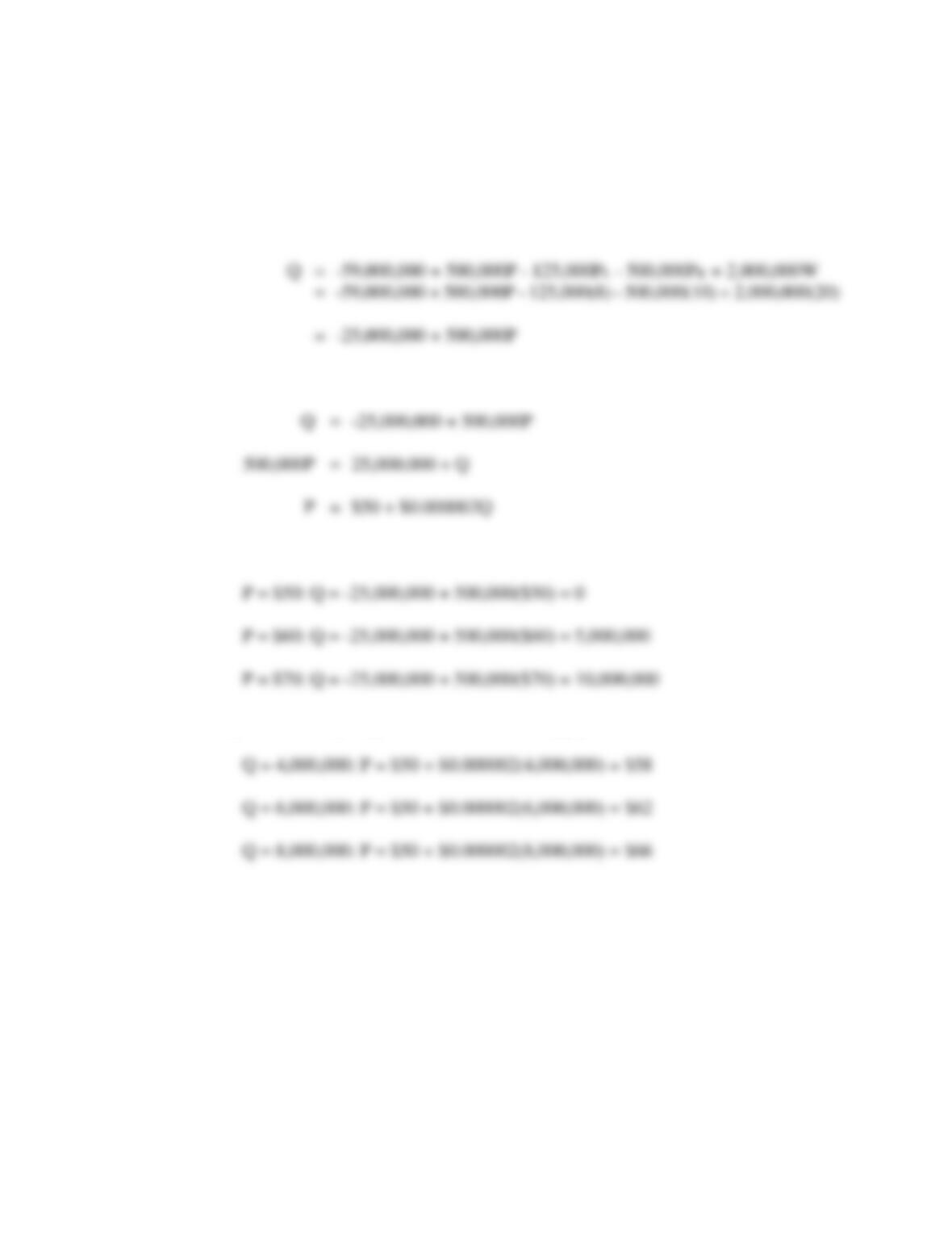
A. With quantity expressed as a function of price, the industry supply curve is:
With price expressed as a function of quantity, the industry supply curve is:
B. Industry supply at each respective price is:
C. The price necessary to generate each level of supply is:
P3.8 Supply Curve Determination. Olympia Natural Resources, Inc., and Yakima Lumber,
Ltd., supply cut logs (raw lumber) to lumber and paper mills located in the Cascades
Mountain region in the state of Washington. Each company has a different marginal
cost of production depending on its own cost of landowner access, labor and other
cutting costs, the distance cut logs must be shipped, and so on. The marginal cost of
producing one unit of output, measured as one thousand board feet of lumber (where
one board foot is one square foot of lumber, one inch thick), is:
MCO = $350 + $0.00005QO (Olympia).
MCY = $150 + $0.0002QY (Yakima).
Demand and Supply 65
The wholesale market for cut logs is vigorously price competitive, and neither firm is
able to charge a premium for its products. Thus, P = MR in this market.
A. Determine the supply curve for each firm. Express price as a function of quantity
and quantity as a function of price. (Hint: Set P = MR = MC to find each firm’s
supply curve.)
D. Determine the industry supply curve when P > $350. To check your answer,
calculate quantity at an industry price of $375 and compare your result with part
B.
P3.8 SOLUTION
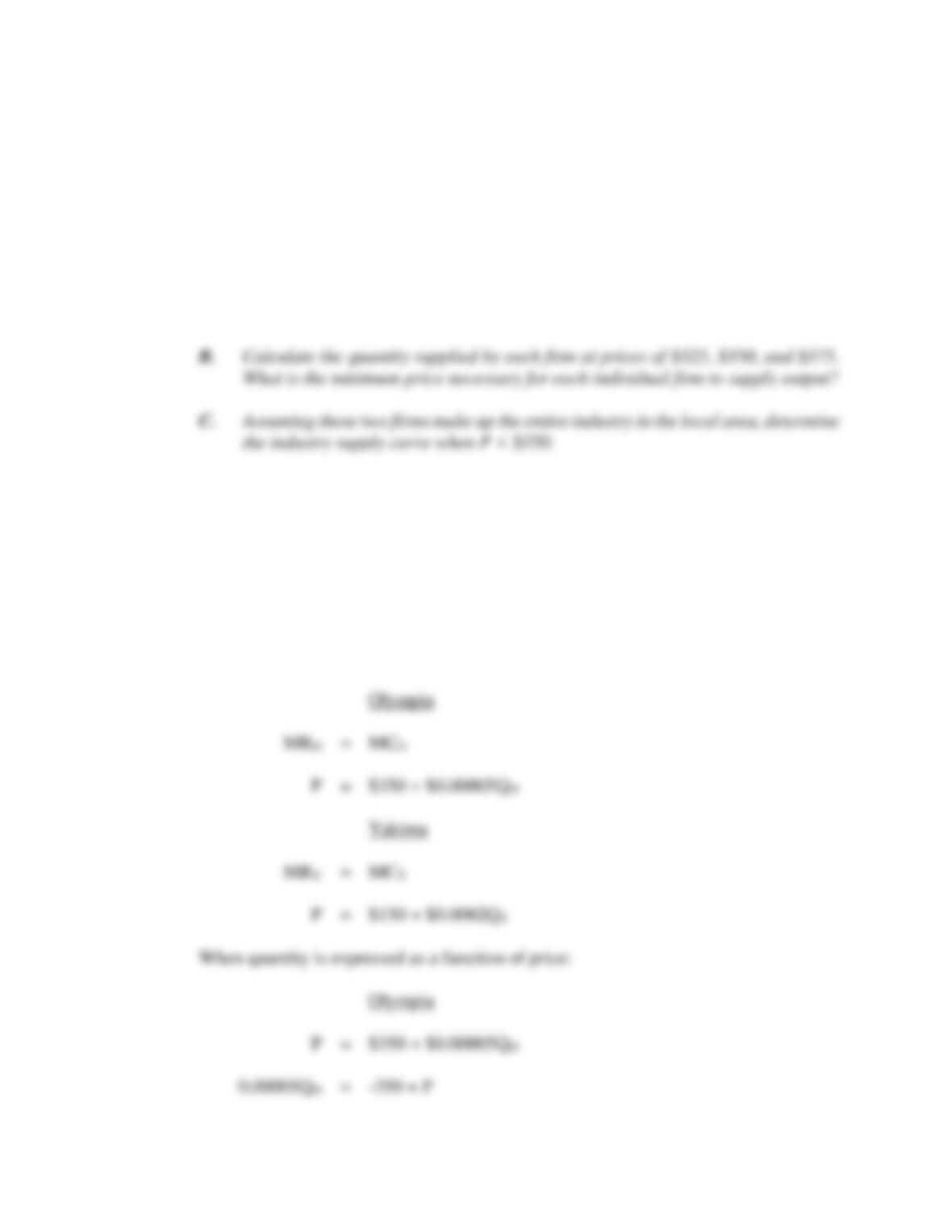
A. Each company will supply output to the point where MR = MC. Because P = MR in this
market, the supply curve for each firm can be written with price as a function of quantity
as:
66 Chapter 3
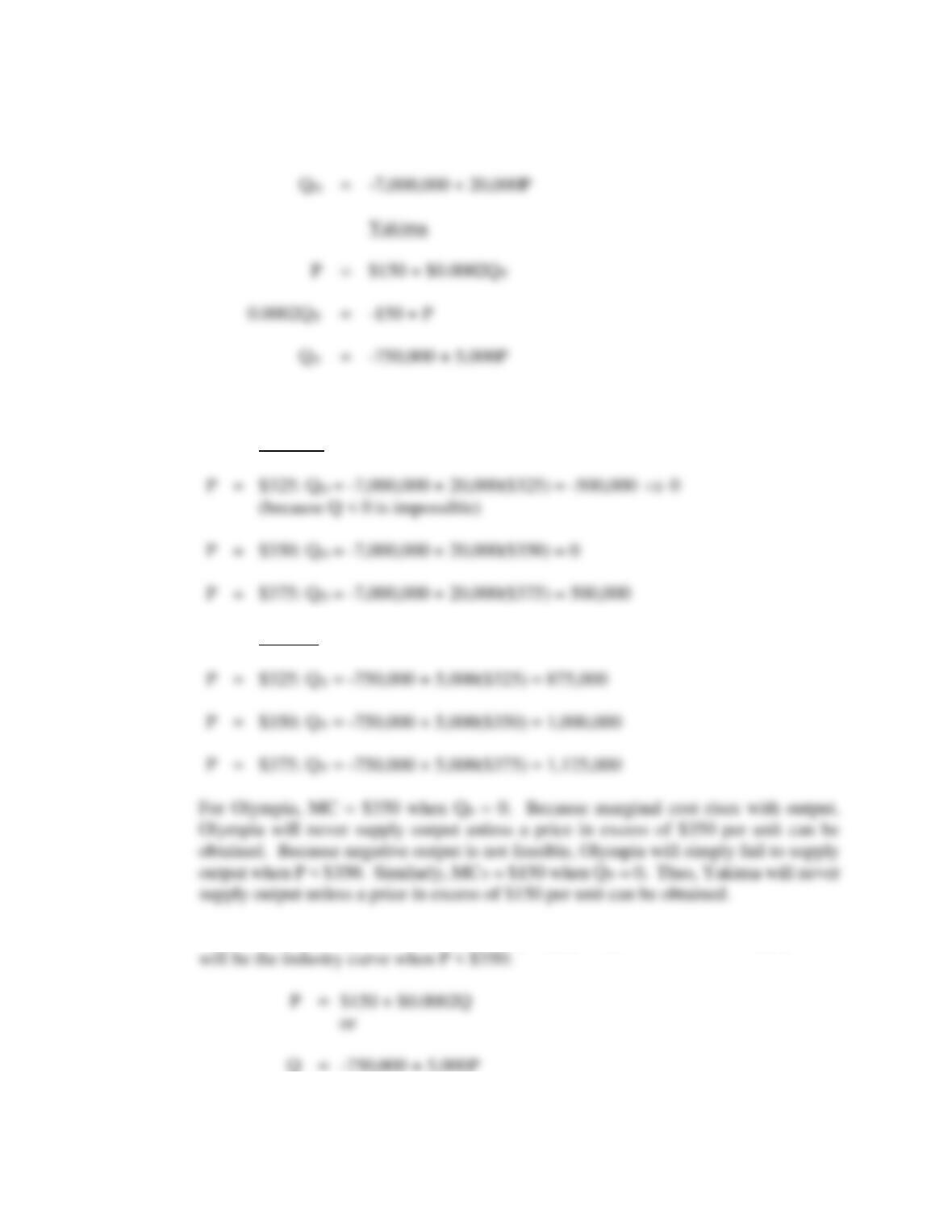
B. The quantity supplied at each respective price is:
Olympia
Yakima
C. When P < $350, only Yakima can profitably supply output. The Yakima supply curve
Demand and Supply 67
D. When P > $350, both Olympia and Yakima can profitably supply output. To derive the
industry supply curve in this circumstance, simply sum the quantities supplied by each
firm:
P3.9 Supply Curve Determination. Cornell Pharmaceutical, Inc., and Penn Medical, Ltd.,
supply generic drugs to treat a wide variety of illnesses. A major product for each
company is a generic equivalent of an antibiotic used to treat postoperative infections.
Proprietary cost and output information for each company reveal the following relations
between marginal cost and output:
MCC = $10 + $0.004QC. (Cornell)
MCP = $8 + $0.008QP. (Penn)
The wholesale market for generic drugs is vigorously price competitive, and neither firm
is able to charge a premium for its products. Thus, P = MR in this market.
B. Calculate the quantity supplied by each firm at prices of $8, $10, and $12. What
is the minimum price necessary for each individual firm to supply output?
68 Chapter 3
C. Assuming these two firms make up the entire industry, determine the industry
supply curve when P < $10.
D. Determine the industry supply curve when P > $10. To check your answer,
calculate quantity at an industry price of $12 and compare your answer with part
B.
P3.9 SOLUTION
Cornell
When quantity is expressed as a function of price:
Demand and Supply 69
B.The quantity supplied at each respective price is:
Cornell
Penn
C. When P < $10, only Penn can profitably supply output. The Penn supply curve will be
D. When P > $10, both Cornell and Penn can profitably supply output. To derive the
70 Chapter 3
P3.10 Market Equilibrium. Eye-de-ho Potatoes is a product of the Coeur d’Alene Growers’
Association. Producers in the area are able to switch back and forth between potato
and wheat production depending on market conditions. Similarly, consumers tend to
regard potatoes and wheat (bread and bakery products) as substitutes. As a result, the
demand and supply of Eye-de-ho Potatoes are highly sensitive to changes in both potato
and wheat prices.
Demand and supply functions for Eye-de-ho Potatoes are as follows:
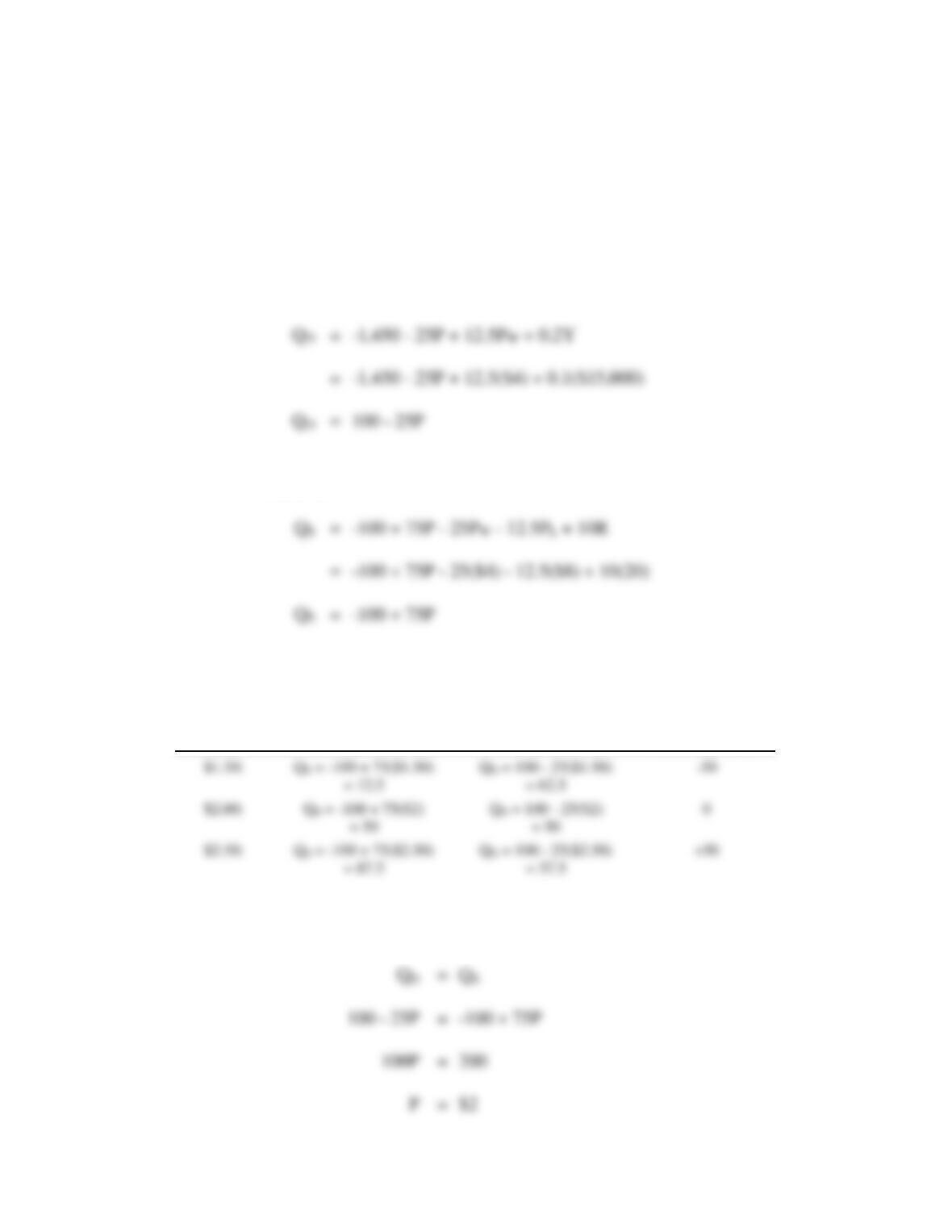
QD = –1,450 – 25P + 12.5PW + 0.1Y, (Demand)
QS = –100 + 75P – 25PW – 12.5PL + 10R, (Supply)
where P is the average wholesale price of Eye-de-ho Potatoes ($ per bushel), PW is the
average wholesale price of wheat ($ per bushel), Y is income (GDP in $ billions), PL is
the average price of unskilled labor ($ per hour), and R is the average annual rainfall
(in inches). Both QD and QS are in millions of bushels of potatoes.
A. When quantity is expressed as a function of price, what are the Eye-de-ho
Potatoes demand and supply curves if PW = $4, Y = $15,000 billion, PL = $8, and
R = 20 inches?
B. Calculate the surplus or shortage of Eye-de-ho Potatoes when P = $1.50, $2, and
$2.50.
C. Calculate the market equilibrium price/output combination.
Demand and Supply 71
P3.10 SOLUTION
A. When quantity is expressed as a function of price, the demand curve for Eye-de-ho
Potatoes is:
When quantity is expressed as a function of price, the supply curve for Eye-de-ho
Potatoes is:
B. The surplus or shortage can be calculated at each price level:
Price
Quantity
Supplied
Quantity
Demanded
Surplus (+) or
Shortage (-)
(1)
(2)
(3)
(4) = (2) – (3)
C. The equilibrium price is found by setting the quantity demanded equal to the quantity
supplied and solving for P:
72 Chapter 3
To solve for Q, set:
Demand and Supply 73
CASE STUDY FOR CHAPTER 3
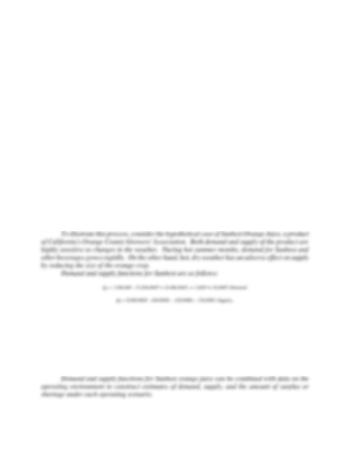
Spreadsheet Analysis of Demand and Supply for Sunbest Orange Juice
Spreadsheet analysis is an appropriate means for studying the demand and supply effects of possible
changes in various exogenous and endogenous variables. Endogenous variables include all
important demand and supply-related factors that are within the control of the firm. Examples
include product pricing, advertising, product design, and so on. Exogenous variables consist of all
significant demand and supply-related influences that are beyond the control of the firm. Examples
include competitor pricing, competitor advertising, weather, general economic conditions, and
related factors.
In comparative statics analysis, the marginal influence on demand and supply of a change in
any one factor can be isolated and studied in depth. The advantage of this approach is that causal
relationships can be identified and responded to, if appropriate. The disadvantage of this marginal
approach is that it becomes rather tedious to investigate the marginal effects of a wide range of
demand and supply influences. It is here that spreadsheet analysis of demand and supply conditions
becomes useful. Using spreadsheet analysis, it is possible to learn the demand and supply
implications of an almost limitless range of operating scenarios. Rather than calculating the effects
of only a few possibilities, it is feasible to consider even rather unlikely outcomes. A complete
picture can be drawn of the firm’s operating environment, and strategies for responding to a host of
operating conditions can be drawn up.
where P is the average wholesale price of Sunbest ($ per case), PS is the average wholesale price of
canned soda ($ per case), Y is disposable income per household ($), T is the average daily high
temperature (degrees), PL is the average price of unskilled labor ($ per hour), and PK is the risk-
adjusted cost of capital (in percent).
During the coming planning period, a wide variety of operating conditions are possible. To gauge
the sensitivity of demand and supply to changes in these operating conditions, a number of scenarios
that employ a range from optimistic to relatively pessimistic assumptions have been drawn up in
Table 3.4.
74 Chapter 3
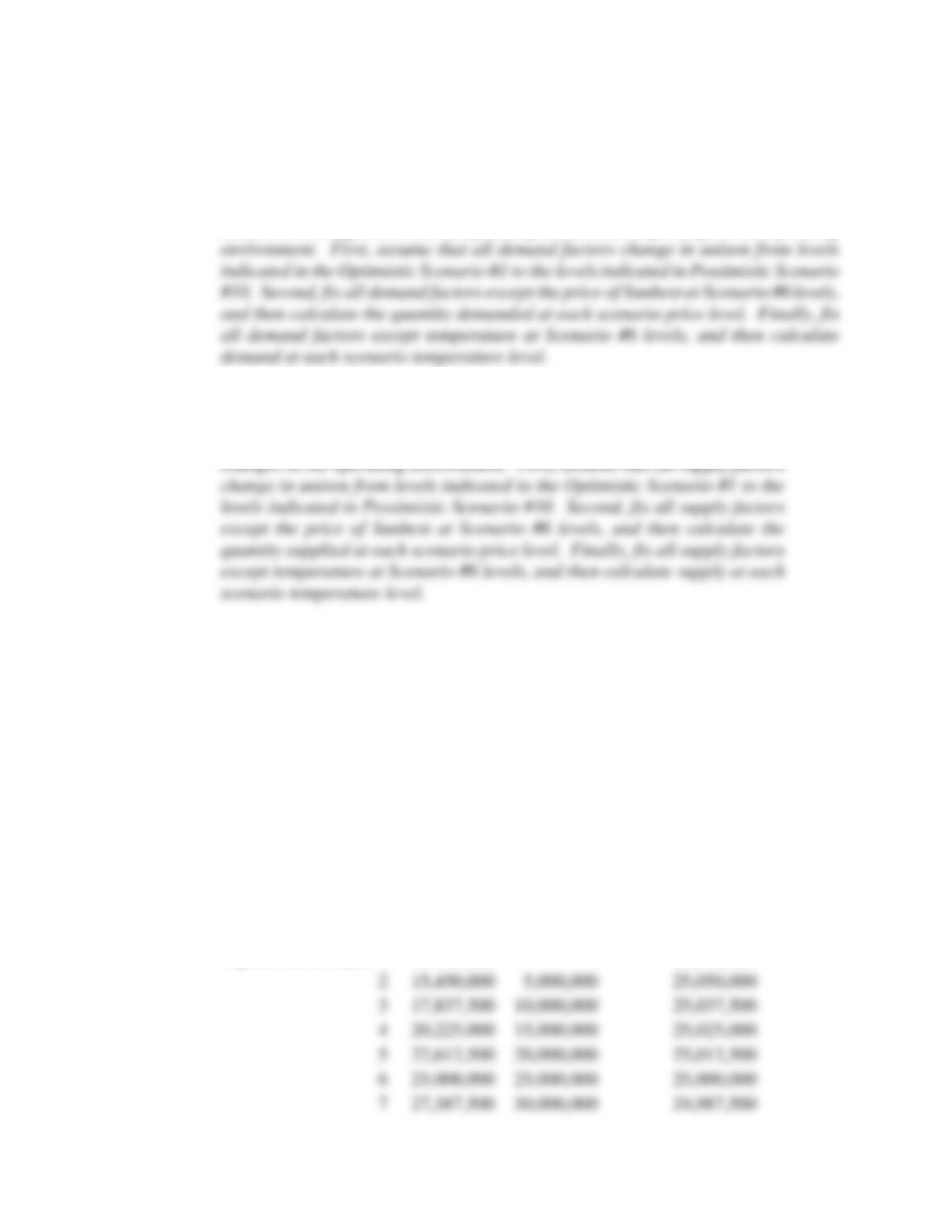
A. Set up a spreadsheet to illustrate the effects of changing economic assumptions on the
demand for Sunbest orange juice. Use the demand function to calculate demand
based on three different underlying assumptions concerning changes in the operating
B. Set up a spreadsheet to illustrate the effects of changing economic
assumptions on the supply of Sunbest orange juice. Use the supply function to
calculate supply based on three different underlying assumptions concerning
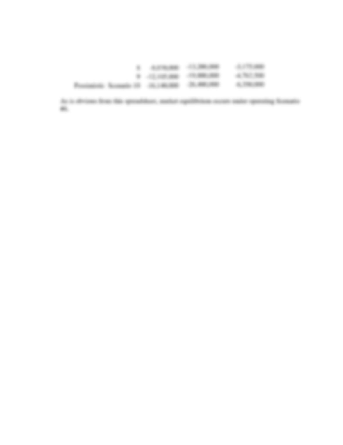
C. Set up a spreadsheet to illustrate the effect of changing economic assumptions on the
surplus or shortage of Sunbest orange juice that results from each scenario detailed
in part A and part B. Which operating scenario results in market equilibrium?
CASE STUDY SOLUTION
A. A spreadsheet that illustrates the effects of changing economic assumptions on the demand
for Sunbest orange juice is as follows:
Operating Environment
for Demand
Demand if
All Factors
Change
(QD)
Quantity
Demanded
if Price
Chgs.
Only(QD)
Demand if Temp.
Chgs. Only (QD)
Optimistic Scenario 1
13,062,500
0
25,062,500
15,450,000
25,050,000
17,837,500
25,037,500
20,225,000
25,025,000
22,612,500
25,012,500
Demand and Supply 75
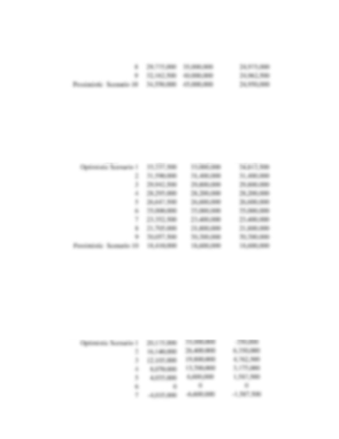
B. A spreadsheet that depicts the consequence of changing economic
assumptions on the supply of Sunbest orange juice is as follows:
Operating Environment
for Supply
Supply if
All Factors
Change
(QS)
Quantity
Supplied if
Price Chgs.
Only(QS)
Supply if
Temp. Chgs.
Only (QS)
C. A spreadsheet illustration of the effect of changing economic assumptions on the surplus
and shortage of Sunbest is:
Operating Environment
for Demand and Supply
Surplus or
Shortage
All Factors
Change
Surplus or
Shortage
Price Chg.
Only
Surplus or
Shortage
Temp. Chg.
Only
76 Chapter 3