30
CHAPTER 3
Demand Curves
A. Summary
This chapter provides a complete development of the demand curve concept.
It begins with the traditional analysis of the effects of changes in income and
prices on the quantities of goods one person demands. Most of the analysis
deals with reactions to price changes: income and substitution effects are
Market demand curves are developed in the second half of Chapter 3 by
summing the individual curves. This construction demonstrates the notion of
price-taking behavior that lies behind such demand curves. The summing
note 8).
The relationship between total expenditures and price elasticity is ana-
lyzed in the chapter, but the concept of marginal revenue is not explicitly in-
B. Lecture and Discussion Suggestions
Comparative statics methodology should be the principal focus of the lecture
for this chapter. It is essential that students understand why one compares
equilibrium (utility-maximizing) positions to analyze behavior. In addition to
Chapter 3: Individual Demand Curves
31
take about one class and would be a useful supplement to material in the text.
A second approach to teaching comparative statics would be to offer an ex-
tended example in lecture. Going over the Lump Sum Principle (Figure 3-6)
should reinforce the distinction between income and substitution effects.
Policy applications of the elasticity concept provide the most interesting
points of departure for discussions based on this chapter. The health insur-
C. Glossary Entries in the Chapter
• Complements
• Consumer Surplus
• Income Effect
• Income Elasticity of Demand
• Increase or Decrease in Demand
• Increase or Decrease in Quantity Demanded
SOLUTIONS TO CHAPTER 3 PROBLEMS
3.1 a. I = $200 S = J.
Chapter 3: Individual Demand Curves
32
c.
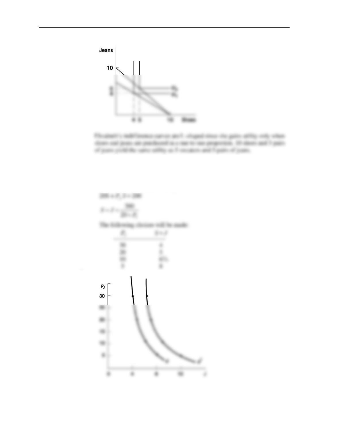
d. The change from
2
U
to
1
U
is entirely attributable to the income effect. There
is no substitution effect due to Elizabeth’s insistence on a fixed proportion of
jeans and shoes.
e. S = J throughout because of her preferences.
f.
Chapter 3: Individual Demand Curves
33
More J is demanded at each price (see graph in part f).
This will shift both demand curves inward.
3.2 a.
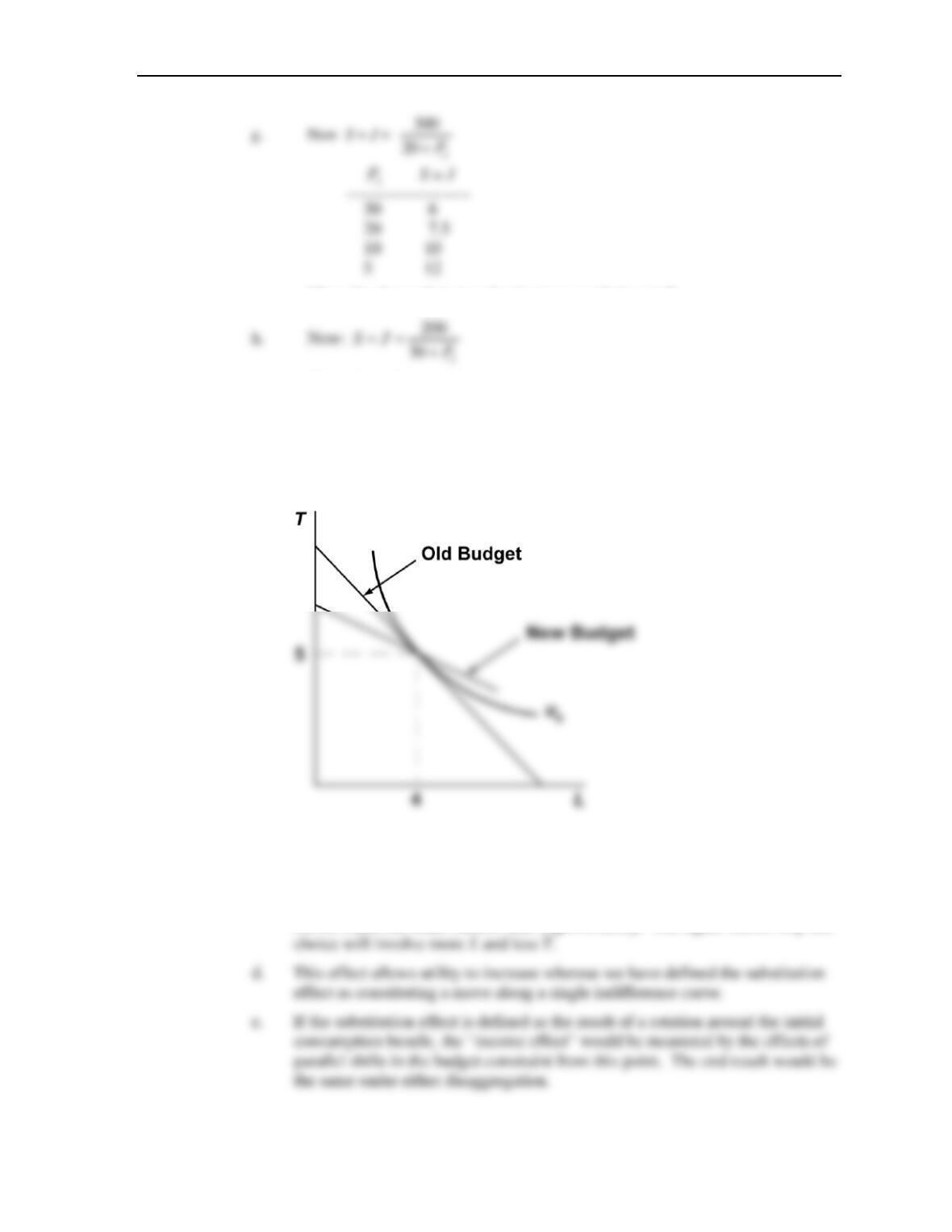
b. These price changes still allow Paula to afford her initial choices. Hence the
budget constraint rotates around this point
( 5, 4)TL==
.
c. Because the new budget constraint is no longer tangent to the indifference
curve, Paula can make choices that improve utility. The figure shows why this
Chapter 3: Individual Demand Curves
34
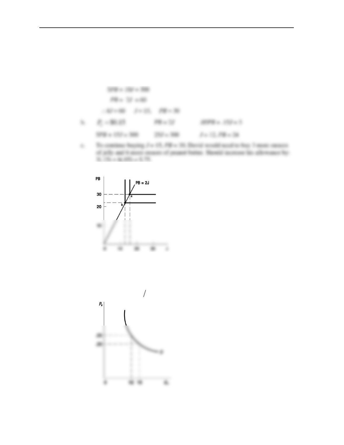
3.3 a. PB = 2J and .05PB + .1J = 3
d.
e. Since David N uses only PB and J to make sandwiches (in fixed proportions),
and because bread is free, it is just as though he buys sandwiches where
2
sandwich PB J
P P P=+
. In part a, PS = .20, QS = 15. In part b, PS = .25, QS = 12.
In general,
3
SS
QP=
Chapter 3: Individual Demand Curves
35
3.4 a. Function is homogeneous because a doubling of I and P leaves Q unchanged
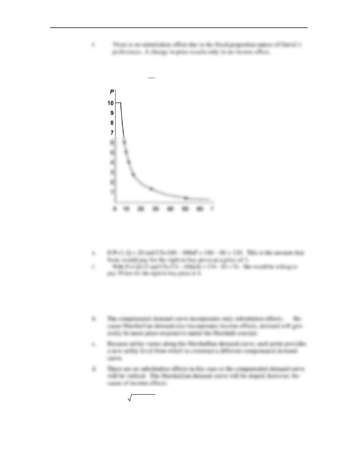
b. Graph of
60
QP
=
c. See graph.
d. Since Q=0 for P>10, CS=0. Equation gives same result.
3.5 a. This is true by definition. The person starts from the same place under either
concept.
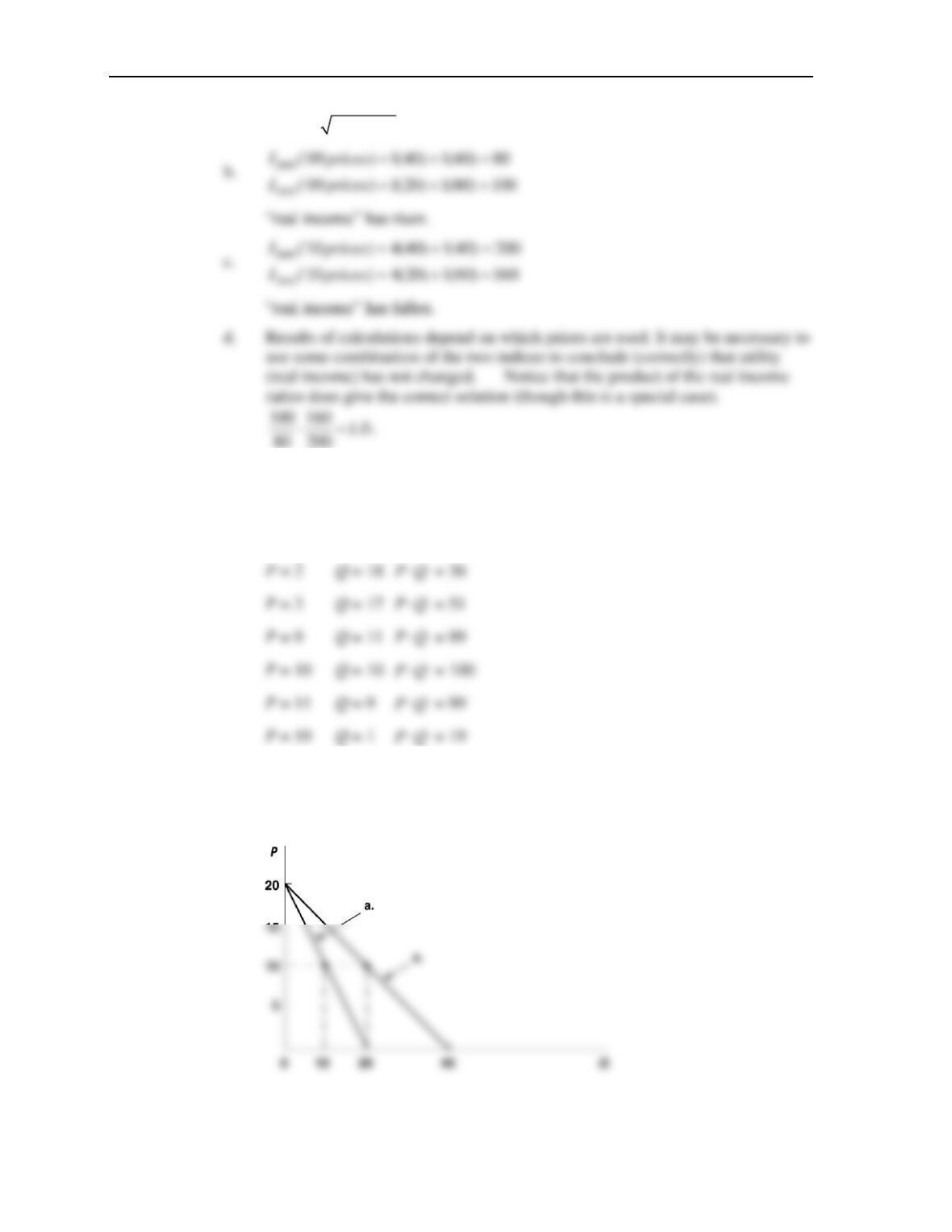
3.6 a. U2009 =
40 40
= 40
Chapter 3: Individual Demand Curves
36
U2010 =
20 80
= 40
3.7 a. Q = 20
b. Q = 0 when P = 20
c. P = 1 Q = 19
PQ
PQ
PQ
PQ
PQ
PQ
= 19
d. Highest total expenditures are 100 when P = 10.
e. Since 40 – 2P = 2(20 – P), Q will be twice as large at each price.
Total expenditures are still as large as possible when P = 10.
Chapter 3: Individual Demand Curves
37
3.8 a. Tom Dick Harry Total
P = 50 0 0 0 0
= 35 30 20 0 50
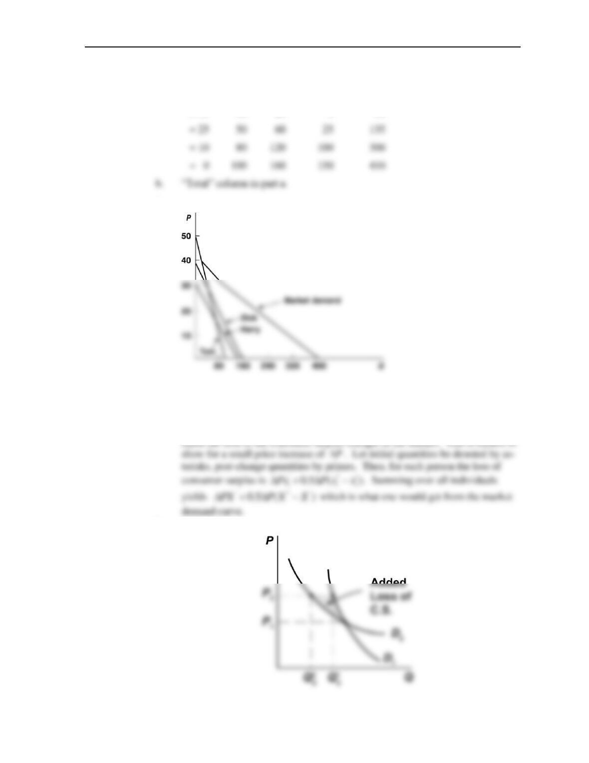
c.
d. Above graph.
3.9 a. Because the market demand curve is the horizontal sum of each individual’s
demand curve, the total area of consumer surplus triangles for each person will
b.
Chapter 3: Individual Demand Curves
38
of the price increase whereas with larger ones they can.
c. This would be literally true only if demand were completely inelastic. With a
more elastic demand total spending total spending may even fall in response to
a price increase though there will still be a loss of consumer surplus.
3.10 a.
a
Pb
−
=
when Q = 0.
b.
**
*
a a Q a Q
YP
b b b b
− − − −
= − = − =
.