19
CHAPTER 3
TEACHING NOTES
For undergraduates, I do not work through most of the derivations in this chapter, at least not in
detail. Rather, I focus on interpreting the assumptions, which mostly concern the population.
Other than random sampling, the only assumption that involves more than population
considerations is the assumption about no perfect collinearity, where the possibility of perfect
collinearity in the sample (even if it does not occur in the population) should be touched on. The
more important issue is perfect collinearity in the population, but this is fairly easy to dispense
with via examples. These come from my experiences with the kinds of model specification
issues that beginners have trouble with.
I have intentionally kept the discussion of multicollinearity to a minimum. This partly indicates
my bias, but it also reflects reality. It is, of course, very important for students to understand the
potential consequences of having highly correlated independent variables. But this is often
beyond our control, except that we can ask less of our multiple regression analysis. If two or
more explanatory variables are highly correlated in the sample, we should not expect to precisely
estimate their ceteris paribus effects in the population.
I do not prove the Gauss-Markov theorem. Instead, I emphasize its implications. Sometimes, and
certainly for advanced beginners, I put a special case of Problem 3.12 on a midterm exam, where

SOLUTIONS TO PROBLEMS
3.1 (i) hsperc is defined so that the smaller it is, the lower the student’s standing in high
school. Everything else equal, the worse the student’s standing in high school, the lower is
his/her expected college GPA.
3.2 (i) Yes. Because of budget constraints, it makes sense that, the more siblings there are in a
family, the less education any one child in the family has. To find the increase in the number of
siblings that reduces predicted education by one year, we solve 1 = .094(sibs), so sibs =
3.3 (i) If adults trade off sleep for work, more work implies less sleep (other things equal), so
1
< 0.
(iii) Since totwrk is in minutes, we must convert five hours into minutes: totwrk =
5(60) = 300. Then sleep is predicted to fall by .148(300) = 44.4 minutes. For a week, 45
minutes less sleep is not an overwhelming change.
(iv) More education implies less predicted time sleeping, but the effect is quite small. If
3.4 (i) A larger rank for a law school means that the school has less prestige; this lowers
starting salaries. For example, a rank of 100 means there are 99 schools thought to be better.
3.5 (i) No. By definition, study + sleep + work + leisure = 168. Therefore, if we change study,
we must change at least one of the other categories so that the sum is still 168.
(ii) From part (i), we can write, say, study as a perfect linear function of the other
22
3.6 Conditioning on the outcomes of the explanatory variables, we have
1
E( )
= E(
ˆ
+
ˆ
3.7 Only (ii), omitting an important variable, can cause bias, and this is true only when the
omitted variable is correlated with the included explanatory variables. The homoskedasticity
3.8 We can use Table 3.2. By definition,
2
> 0, and by assumption, Corr(x1,x2) < 0.
3.9 (i)
1
< 0 because more pollution can be expected to lower housing values; note that
1
is
the elasticity of price with respect to nox.
2
2
is probably positive because rooms roughly
measures the size of a house. (However, it does not allow us to distinguish homes where each
3.10 (i) Because
1
x
is highly correlated with
2
x
and
3
x
, and these latter variables have large
partial effects on y, the simple and multiple regression coefficients on
1
x
can differ by large
23
).
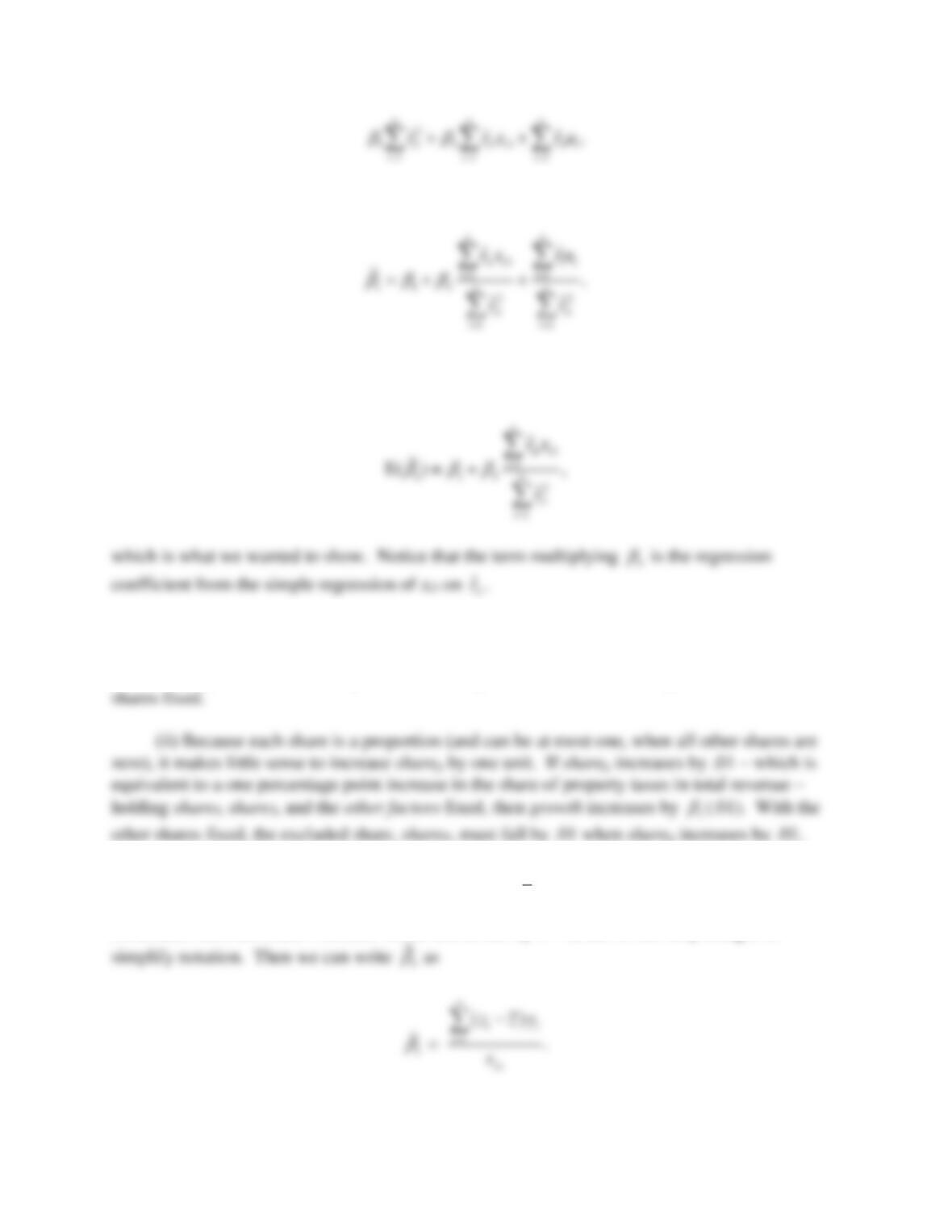
3.11 From equation (3.22) we have
where the
1
ˆ
i
r
are defined in the problem. As usual, we must plug in the true model for yi:
24
Putting these back over the denominator gives
Conditional on all sample values on x1, x2, and x3, only the last term is random due to its
dependence on ui. But E(ui) = 0, and so
3.12 (i) The shares, by definition, add to one. If we do not omit one of the shares then the
equation would suffer from perfect multicollinearity. The parameters would not have a ceteris
paribus interpretation, as it is impossible to change one share while holding all of the other
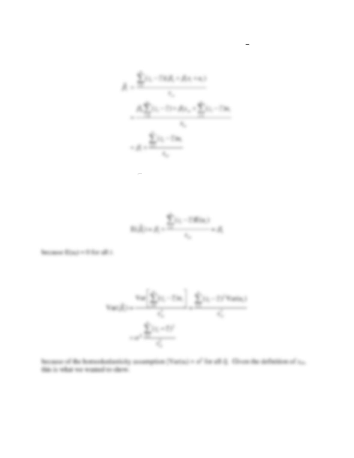
3.13 (i) For notational simplicity, define szx =
1
( ) ;
n
ii
i
z z x
=
−
this is not quite the sample
covariance between z and x because we do not divide by n – 1, but we are only using it to
25
This is clearly a linear function of the yi: take the weights to be wi = (zi −
z
)/szx. To show
unbiasedness, as usual we plug yi =
0
+
1
xi + ui into this equation, and simplify:
where we use the fact that
1
()
n
i
i
zz
=
−
= 0 always. Now szx is a function of the zi and xi and the
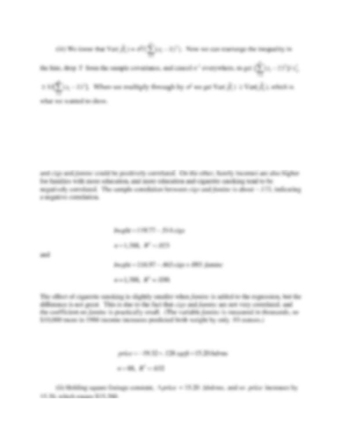
expected value of each ui is zero conditional on all zi and xi in the sample. Therefore, conditional
on these values,
(ii) From the fourth equation in part (i) we have (again conditional on the zi and xi in the
sample),
26
SOLUTIONS TO COMPUTER EXERCISES
C3.1 (i) Probably
2
> 0, as more income typically means better nutrition for the mother and
better prenatal care.
(ii) On the one hand, an increase in income generally increases the consumption of a good,
(iii) The regressions without and with faminc are
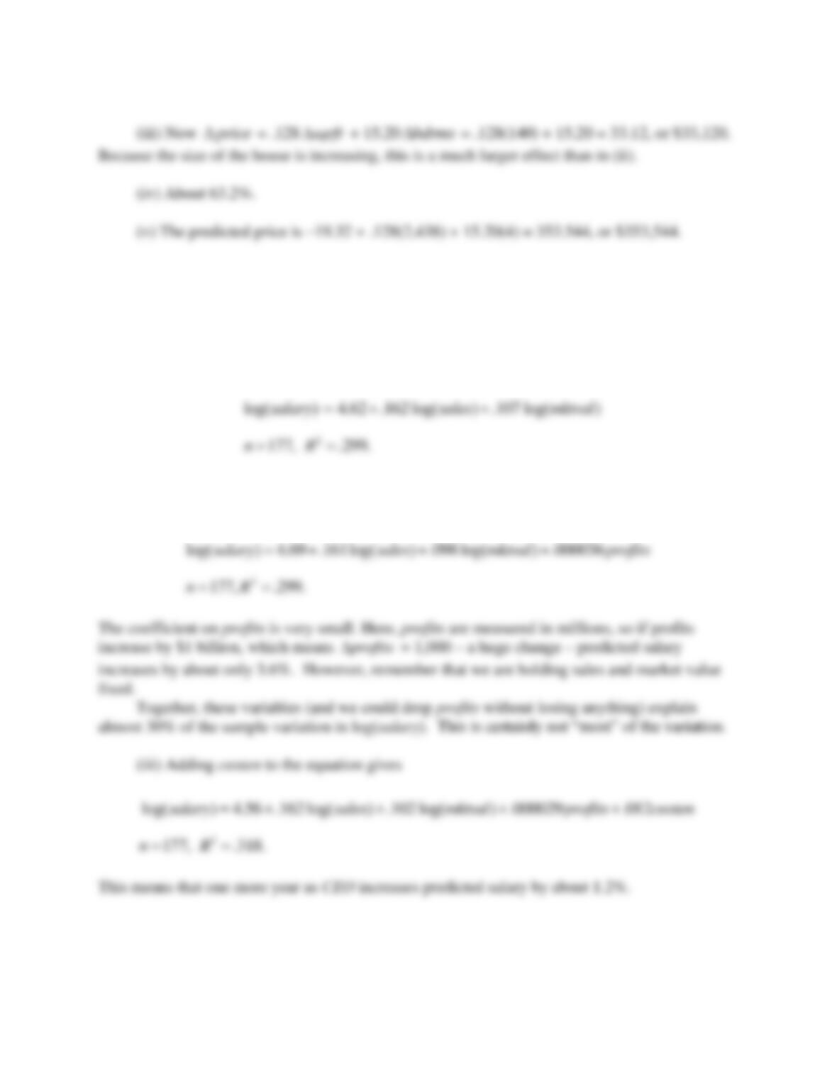
C3.2 (i) The estimated equation is
15.20, which means $15,200.
27
(vi) From part (v), the estimated value of the home based only on square footage and
number of bedrooms is $353,544. The actual selling price was $300,000, which suggests the
buyer underpaid by some margin. But, of course, there are many other features of a house (some
that we cannot even measure) that affect price, and we have not controlled for these.
C3.3 (i) The constant elasticity equation is
(ii) We cannot include profits in logarithmic form because profits are negative for nine of
the companies in the sample. When we add it in levels form we get
(iv) The sample correlation between log(mktval) and profits is about .78, which is fairly
high. As we know, this causes no bias in the OLS estimators, although it can cause their
variances to be large. Given the fairly substantial correlation between market value and firm
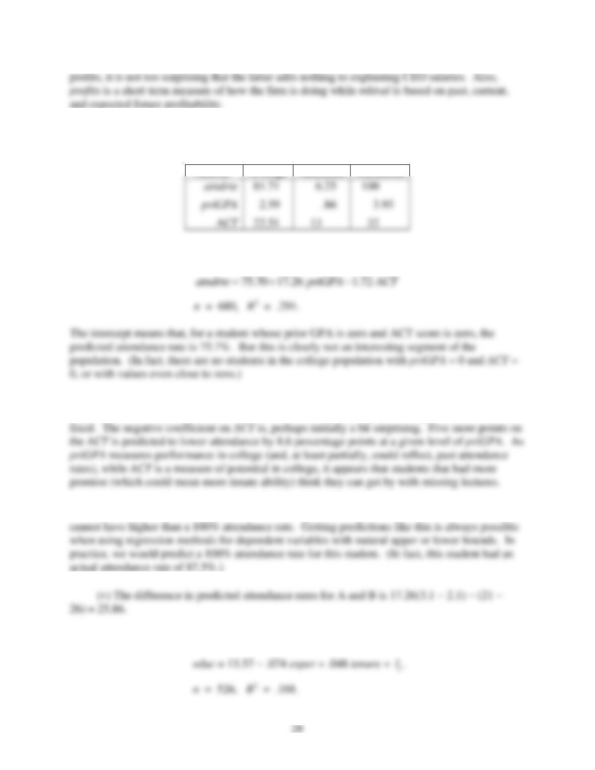
C3.4 (i) The minimum, maximum, and average values for these three variables are given in the
table below:
Variable
Average
Minimum
Maximum
22.51
13
32
(ii) The estimated equation is
(iii) The coefficient on priGPA means that, if a student’s prior GPA is one point higher
(say, from 2.0 to 3.0), the attendance rate is about 17.3 percentage points higher. This holds ACT
(iv) We have
atndrte
= 75.70 + 17.267(3.65) – 1.72(20)
104.3. Of course, a student
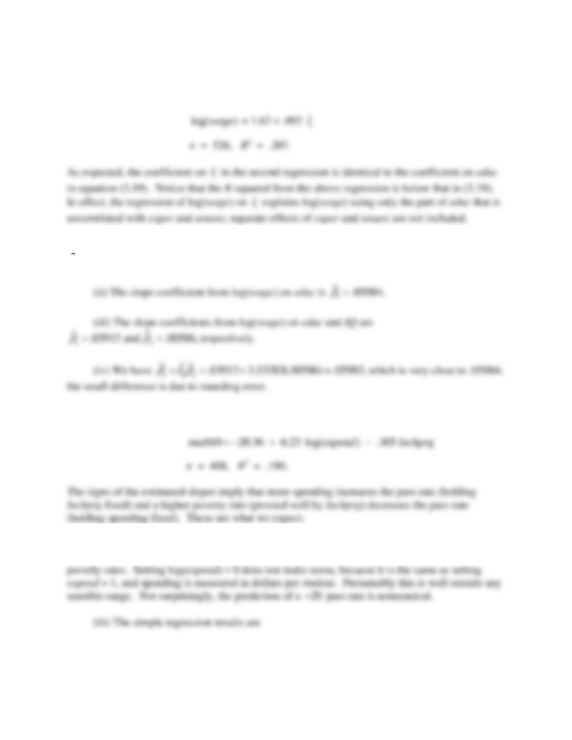
C3.5 The regression of educ on exper and tenure yields
29
Now, when we regress log(wage) on
1
ˆ
r
we obtain
C3.6 (i) The slope coefficient from the regression IQ on educ is (rounded to five decimal places)
13.53383.
=
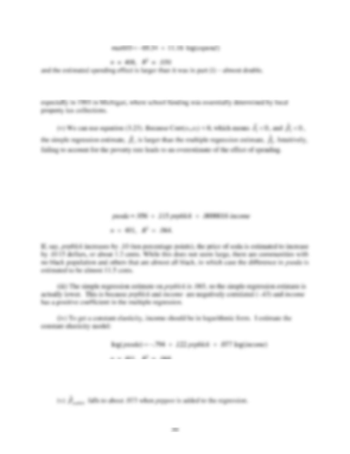
C3.7 (i) The results of the regression are
(ii) As usual, the estimated intercept is the predicted value of the dependent variable when
all regressors are set to zero. Setting lnchprg = 0 makes sense, as there are schools with low
(iv) The sample correlation between lexpend and lnchprg is about
.19−
, which means that,
on average, high schools with poorer students spent less per student. This makes sense,
C3.8 (i) The average of prpblck is .113 with standard deviation .182; the average of income is
47,053.78 with standard deviation 13,179.29. It is evident that prpblck is a proportion and that
income is measured in dollars.
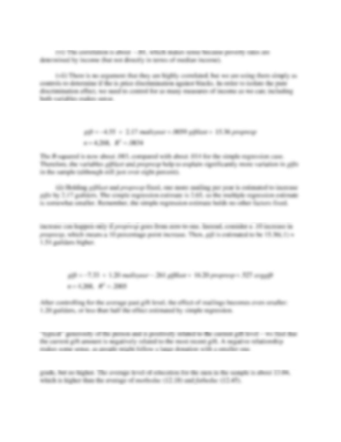
(ii) The results from the OLS regression are
n = 401, R2 = .068.
If prpblck increases by .20, log(psoda) is estimated to increase by .20(.122) = .0244, or about
2.44 percent.
31
C3.9 (i) The estimated equation is
(iii) Because propresp is a proportion, it makes little sense to increase it by one. Such an
(iv) The estimated equation is
(v) After controlling for the average of past gifts – which we can view as measuring the
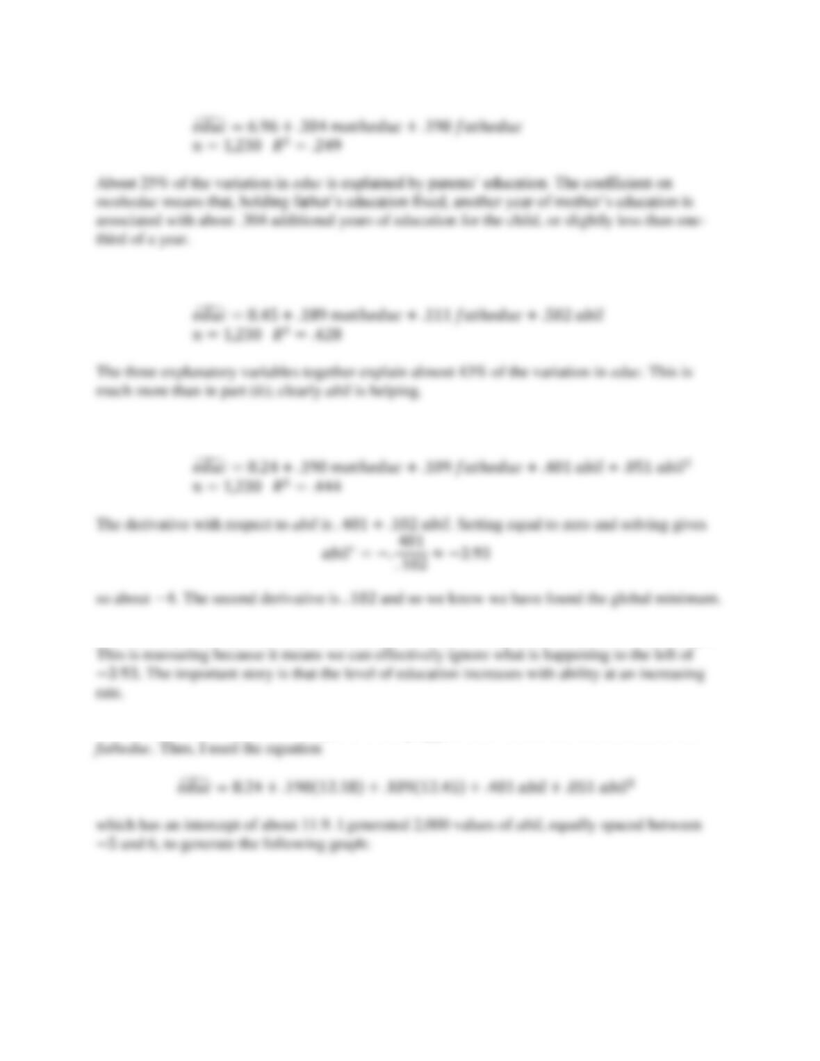
C3.10 (i) The variable educ ranges from 6 to 20. Out of 1,230 men, 512, or 41.63, completed 12th
(ii) The regression results are
32
(iii) When abil is added to the regression we get
(iv) When 𝑎𝑏𝑖𝑙2 is added to the regression the estimated equation is
(v) Out of 1,230 men, only 15 have 𝑎𝑏𝑖𝑙 < −3.93, or only about 1.2 percent of the sample.
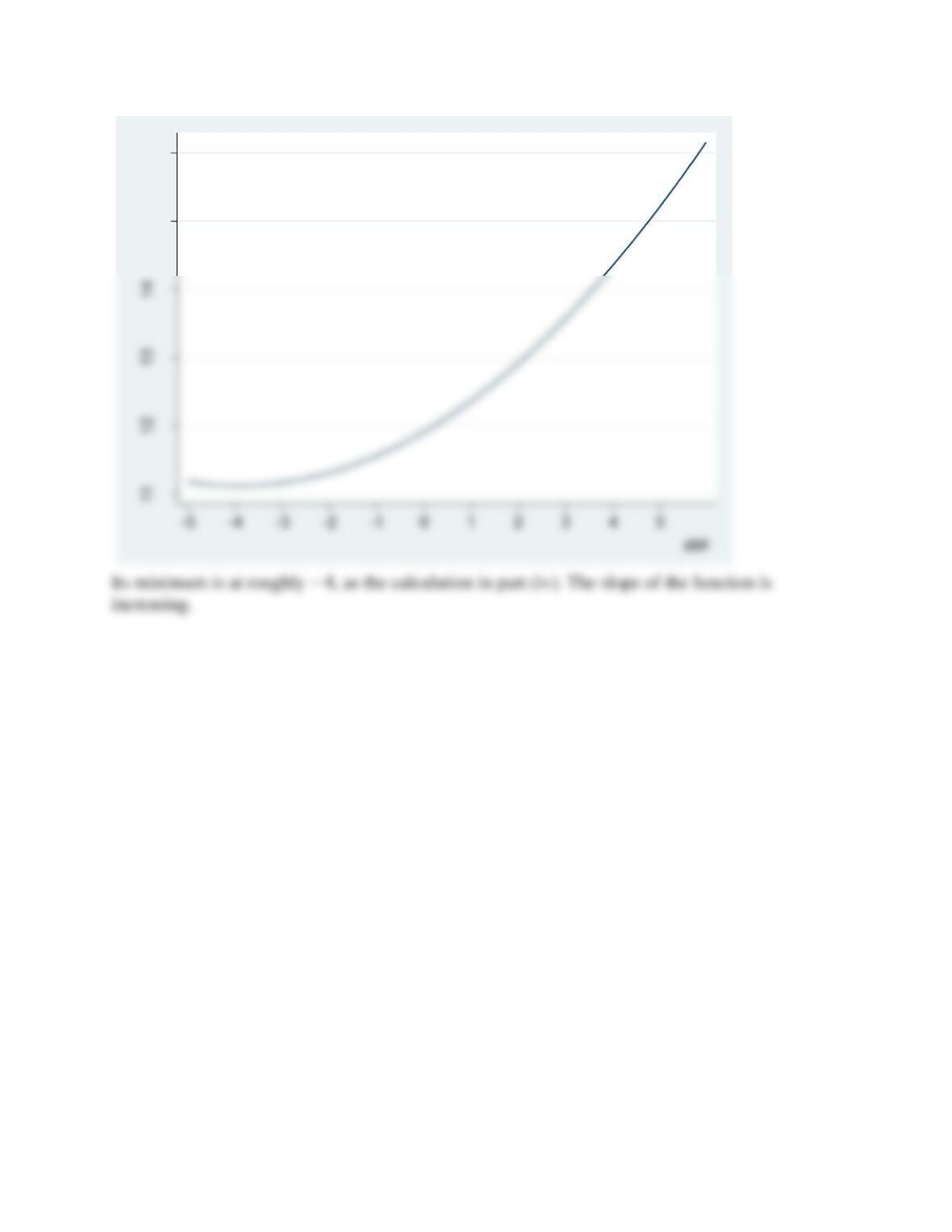
(vi) I used the equation from part (iv) and plugged in the mean values for motheduc and
33
educhat