Chapter 3
DEMAND AND SUPPLY
QUESTIONS AND ANSWERS
Q3.1 What key ingredients are necessary for the creation of economic demand?
Q3.1 ANSWER
Two basic conditions must be met before economic demand is created. First, there must
Q3.2 Memory chip maker Micron Technology Inc. enjoys strong demand for its products from
manufacturers of computers and intelligent electronics. Describe the difference between
direct demand and derived demand.
Q3.2 ANSWER
Direct demand is consumption demand for goods and services. Direct demand is
Q3.3 The Ford Escape Hybrid is the first gas-electric hybrid SUV produced and sold in North
America. How would Ford estimate the demand influence of growing environmental
awareness by consumers?
Q3.3 ANSWER
Variables are included in a demand function because they are thought to affect the
quantity of a product that will be purchased. Some variables such as income, education,
Demand and Supply 49
Q3.4 The Energy Department estimates that domestic demand for natural gas will grow by
more than 40% between now and 2025. Distinguish between a demand function and a
demand curve. What is the difference between a change in the quantity demanded and a
shift in the demand curve?
Q3.4 ANSWER
A demand function is a statement of the relation between the demand for a product and
Q3.5 What key ingredients are necessary for the creation of economic supply?
Q3.5 ANSWER
Two basic conditions must be satisfied before economic supply can be created. First,
Q3.6 The United States is a big exporter of animal feeds, corn, meat, fruits, vegetables and
other agricultural commodities. Explain how foreign trade affects the domestic supply
of such products.
Q3.6 ANSWER
The supply function includes all of those factors with an important direct influence on
the quantity supplied. As the price of a product rises, supply will also rise as producers
seek to earn a profit by meeting consumer demands. When the price of a product falls,
50 Chapter 3
Q3.7 Distinguish between a supply function and a supply curve. What is the difference
between a change in the quantity supplied and a shift in the supply curve?
Q3.7 ANSWER
A supply function is a statement of the relation between the supply of a product and all
Q3.8 “Dynamic rather than static demand and supply conditions are typically observed in
real-world markets. Therefore, comparative statics analysis has only limited value.”
Discuss this statement.
Q3.8 ANSWER
The statement “all else equal” seldom holds in dynamic real-world markets.
Nevertheless, comparative statics analysis provides a useful guide to managerial
Q3.9 Contrast the supply and demand conditions for new Ph.D.’s in economics and
accounting. Why do such large differences in starting salaries seem to persist over
time?
Demand and Supply 51
Q3.9 ANSWER
Economics, like psychology, has long been regarded as an important component of a
well-balanced liberal arts education. As such, the subject of economics is exposed to a
large number of undergraduate students early in their academic career and is typically a
popular major field of study. The importance of economics in everyday life and
Q3.10 Suppose the personal income tax was replaced with a national sales tax. How would
this affect aggregate supply, aggregate demand and interest rates?
Q3.10 ANSWER
Economists, like the late Milton Friedman, sometimes favor replacing the personal
52 Chapter 3
SELF-TEST PROBLEMS AND SOLUTIONS
ST3.1 Demand and Supply Curves. The following relations describe demand and supply
conditions in the lumber/forest products industry
QD = 80,000 – 20,000P (Demand)
QS = -20,000 + 20,000P (Supply)
where Q is quantity measured in thousands of board feet (one square foot of lumber, one
inch thick) and P is price in dollars.
A. Set up a spreadsheet to illustrate the effect of price (P), on the quantity supplied
(QS), quantity demanded (QD), and the resulting surplus (+) or shortage (-) as
represented by the difference between the quantity supplied and the quantity
demanded at various price levels. Calculate the value for each respective variable
based on a range for P from $1.00 to $3.50 in increments of 10¢ (i.e., $1.00,
$1.10, $1.20, . . . $3.50).
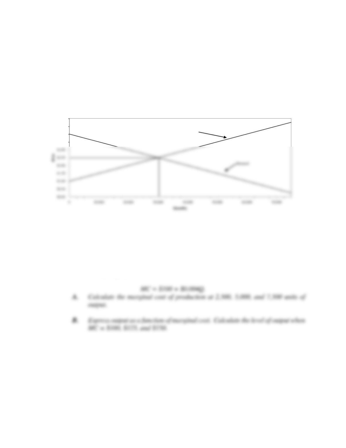
B. Using price (P) on the vertical or y-axis and quantity (Q) on the horizontal or x-
axis, plot the demand and supply curves for the lumber/forest products industry
over the range of prices indicated previously.
ST3.1 SOLUTION
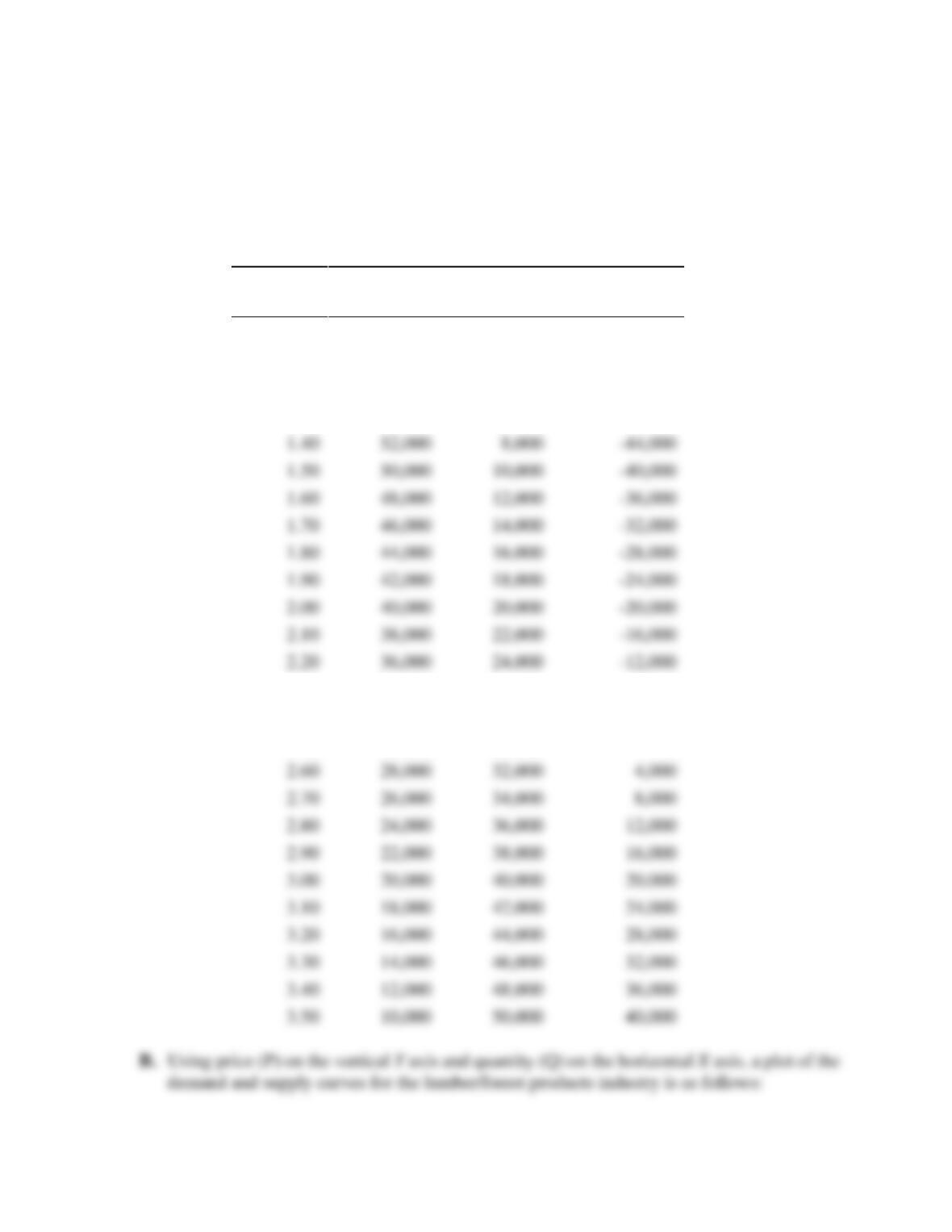
A. A table or spreadsheet that illustrates the effect of price (P), on the quantity supplied
(QS), quantity demanded (QD), and the resulting surplus (+) or shortage (-) as
Demand and Supply 53
Lumber and Forest Industry Supply
and Demand Relationships
Price
Quantity
Demanded
Quantity
Supplied
Surplus (+) or
Shortage (-)
$1.00
60,000
0
-60,000
1.10
58,000
2,000
-56,000
1.20
56,000
4,000
-52,000
1.30
54,000
6,000
-48,000
2.30
34,000
26,000
-8,000
2.40
32,000
28,000
-4,000
2.50
30,000
30,000
0
2.60
28,000
32,000
2.70
26,000
34,000
2.80
24,000
36,000
2.90
22,000
38,000
3.00
20,000
40,000
3.10
18,000
42,000
3.20
16,000
44,000
3.30
14,000
46,000
3.40
12,000
48,000
3.50
10,000
50,000
1.40
52,000
8,000
-44,000
1.50
50,000
10,000
-40,000
1.60
48,000
12,000
-36,000
1.70
46,000
14,000
-32,000
1.80
44,000
16,000
-28,000
1.90
42,000
18,000
-24,000
2.00
40,000
20,000
-20,000
2.10
38,000
22,000
-16,000
54 Chapter 3
ST3.2 Supply Curve Determination. Information Technology, Inc., is a supplier of math
coprocessors (computer chips) used to speed the processing of data for analysis on
personal computers. Based on an analysis of monthly cost and output data, the
company has estimated the following relation between the marginal cost of production
and monthly output:
C. Calculate the profit-maximizing level of output if wholesale prices are stable in the
industry at $150 per chip and, therefore, P = MR = $150.
D. Derive the company’s supply curve for chips assuming P = MR. Express price as
a function of quantity and quantity as a function of price.
ST3.2 SOLUTION
Lumber and Forest Industry Supply and Demand Relationships
$3.50
$4.00
$4.50
$5.00
Supply
Demand and Supply 55
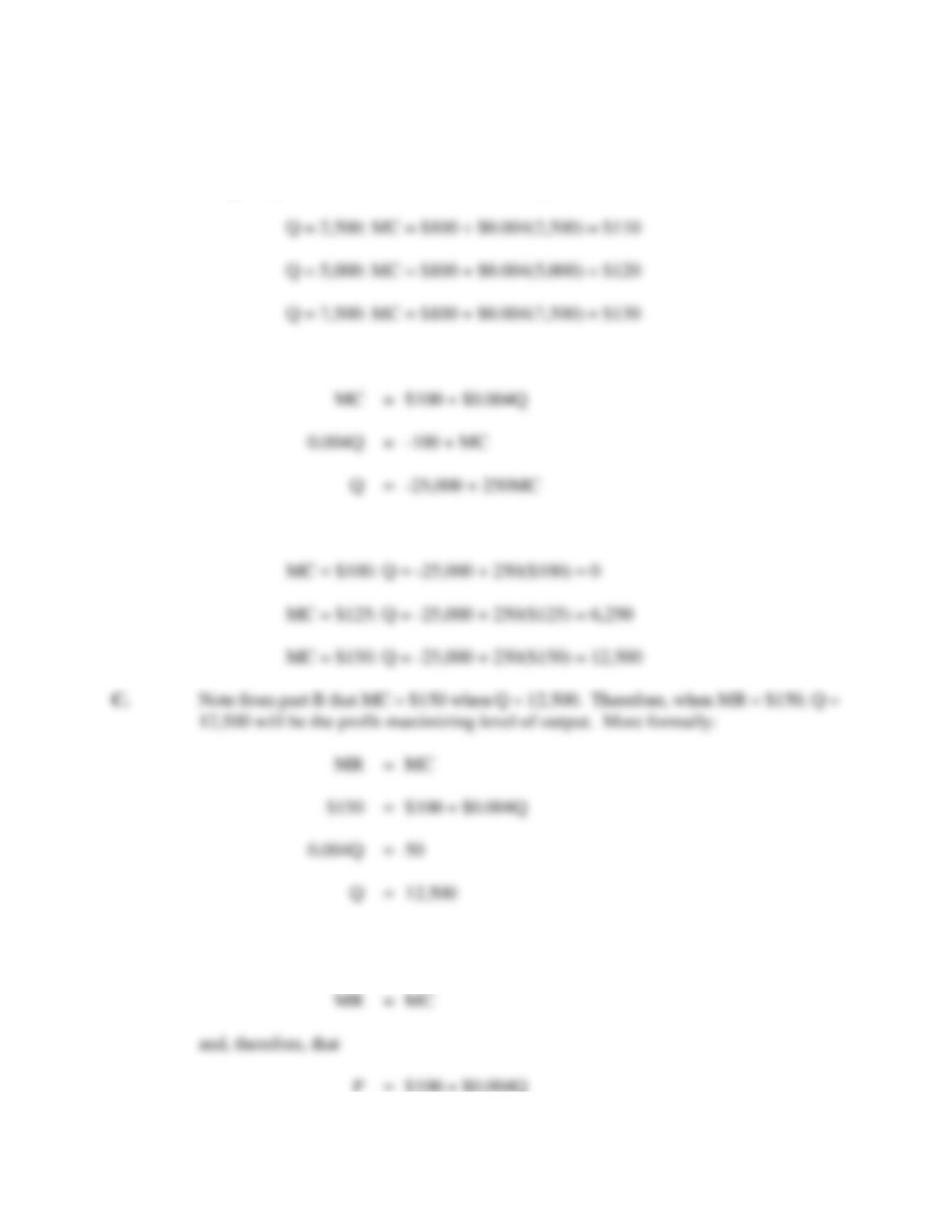
A. Marginal production costs at each level of output are:
B. When output is expressed as a function of marginal cost:
The level of output at each respective level of marginal cost is:
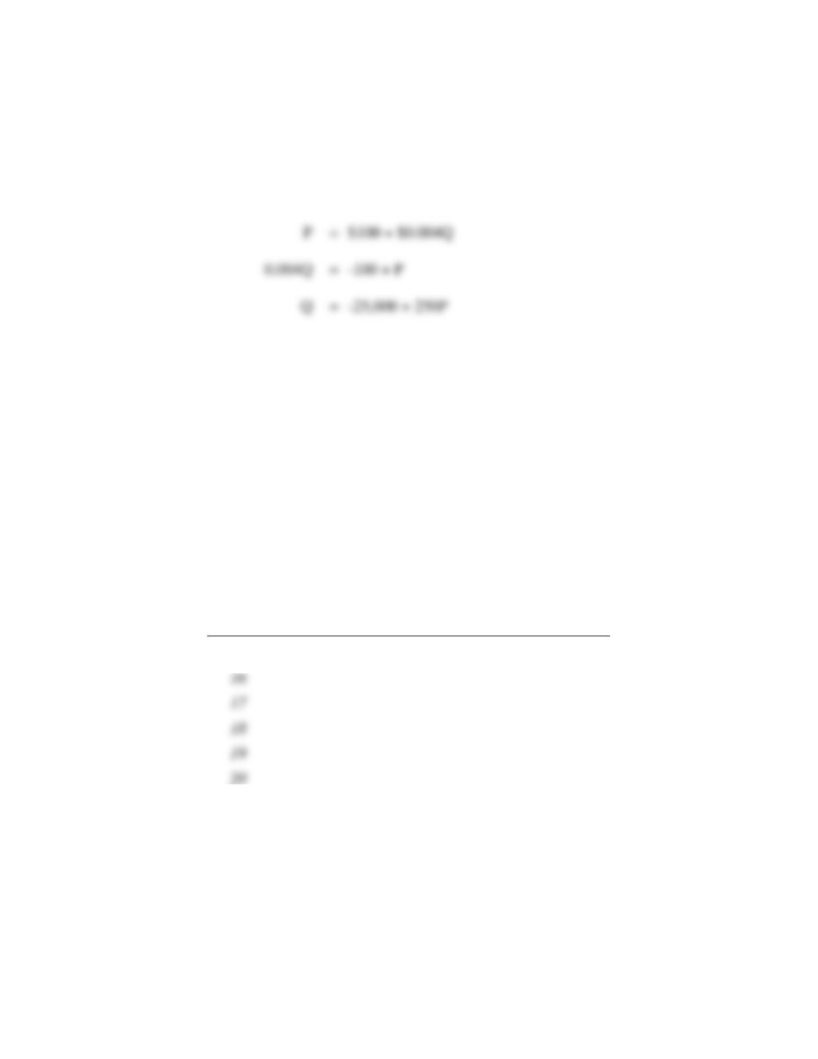
D. Because prices are stable in the industry, P = MR, this means that the company will
supply chips at the level of output where
56 Chapter 3
This is the supply curve for math chips, where price is expressed as a function of
quantity. When quantity is expressed as a function of price:
PROBLEMS AND SOLUTIONS
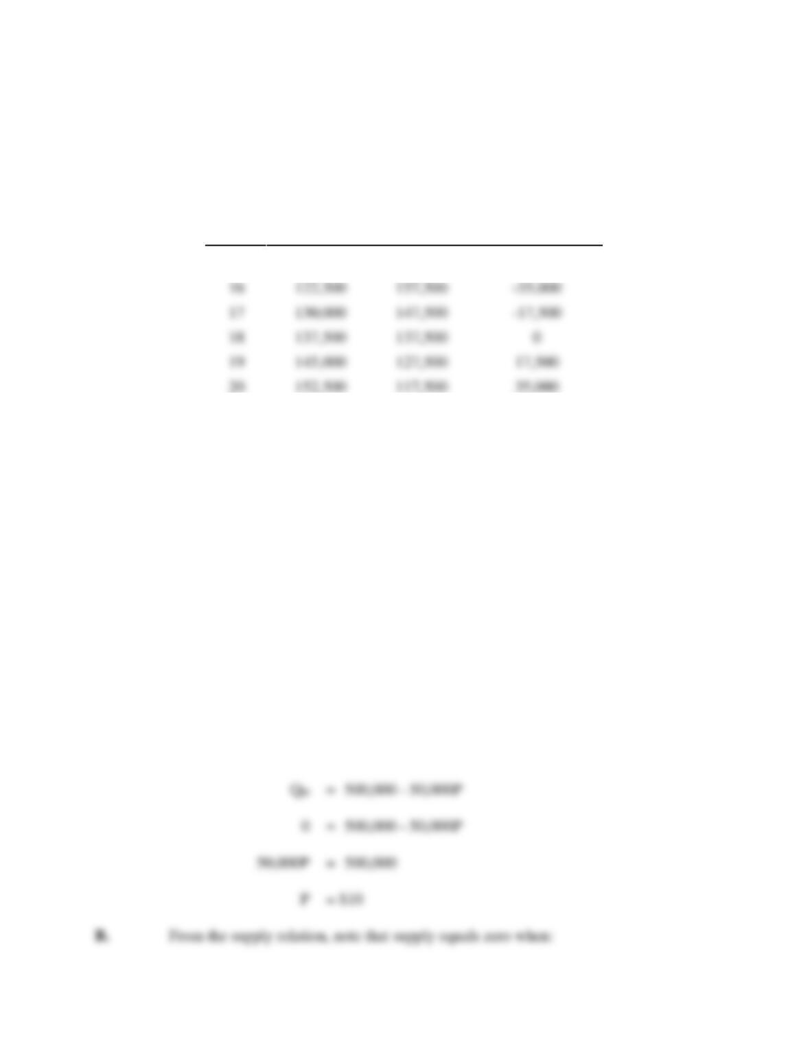
P3.1 Demand and Supply Curves. The following relations describe monthly demand and
supply conditions in the metropolitan area for recyclable aluminum
QD = 317,500 – 10,000P (Demand)
QS = 2,500 + 7,500P, (Supply)
where Q is quantity measured in pounds of scrap aluminum and P is price in cents.
Complete the following table:
Price
(1)
Quantity
Supplied
(2)
Quantity
Demanded
(3)
Surplus (+) or
Shortage (-)
(4) = (2) – (3)
15¢
Demand and Supply 57
P3.1 SOLUTION
Price
(1)
Quantity
Supplied
(2)
Quantity
Demanded
(3)
Surplus (+) or
Shortage (-)
(4) = (2) – (3)
15¢
115,000
167,500
-52,500
P3.2 Demand and Supply Curves. The following relations describe monthly demand and
supply relations for dry cleaning services in the metropolitan area:
QD = 500,000 – 50,000P (Demand)
QS = -100,000 + 100,000P (Supply)
where Q is quantity measured by the number of items dry cleaned per month and P is
average price in dollars.
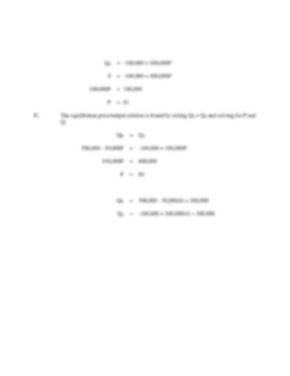
A. At what average price level would demand equal zero?
B. At what average price level would supply equal zero?
C. Calculate the equilibrium price/output combination.
P3.2 SOLUTION
A. From the demand relation, note that demand equals zero when:
58 Chapter 3
Notice that QD = QS = 300,000 at this price because:
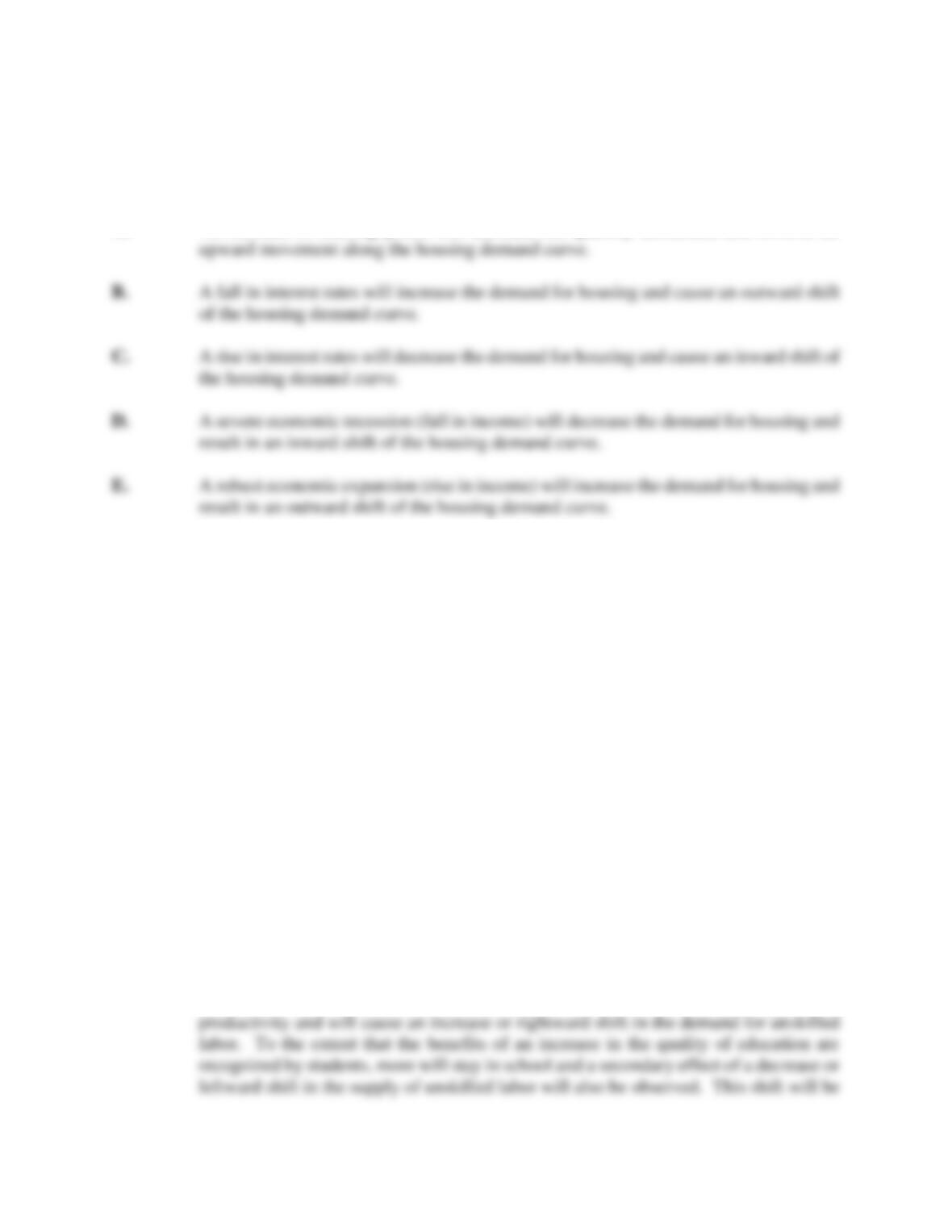
P3.3 Demand Analysis. The demand for housing is often described as being highly cyclical
and very sensitive to housing prices and interest rates. Given these characteristics,
describe the effect of each of the following in terms of whether it would increase or
decrease the quantity demanded or the demand for housing. Moreover, when price is
expressed as a function of quantity, indicate whether the effect of each of the following is
an upward or downward movement along a given demand curve or involves an outward
or inward shift in the relevant demand curve for housing. Explain your answers.
A. An increase in housing prices
B. A fall in interest rates
C. A rise in interest rates
D. A severe economic recession
E. A robust economic expansion
Demand and Supply 59
P3.3 SOLUTION
A. An increase in housing prices will decrease the quantity demanded and involve an
P3.4 Demand and Supply Curves. Demand and supply conditions in the market for unskilled
labor are important concerns to business and government decision makers. Consider
the case of a federally mandated minimum wage set above the equilibrium, or market
clearing, wage level. Some of the following factors have the potential to influence the
demand or quantity demanded of unskilled labor. Influences on the supply or quantity
supplied may also result. Holding all else equal, describe these influences as increasing
or decreasing, and indicate the direction of the resulting movement along or shift in the
relevant curve(s).
A. An increase in the quality of secondary education.
B. A rise in welfare benefits.
C. An increase in the popularity of self-service gas stations, car washes, and so on.
D. A fall in interest rates.
E. An increase in the minimum wage.
P3.4 SOLUTION
A. An increase in the quality of secondary education has the effect of increasing worker
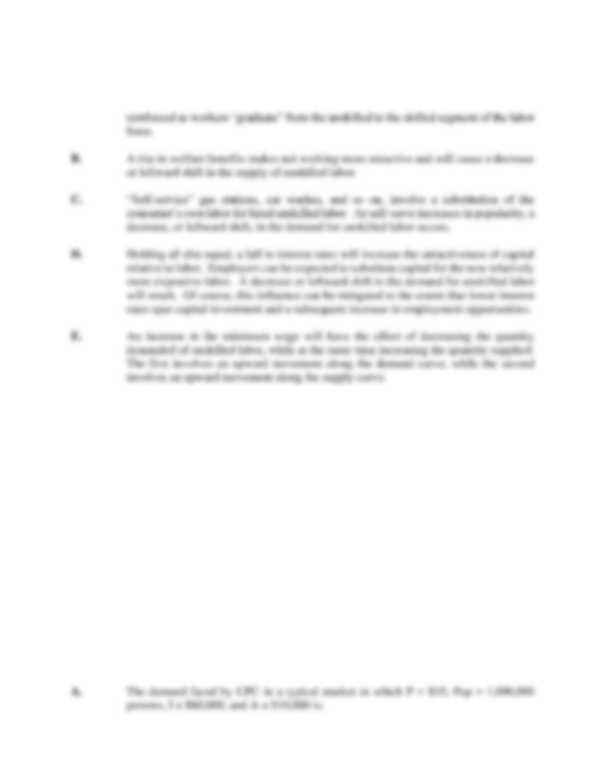
60 Chapter 3
P3.5 Demand Function. The Creative Publishing Company (CPC) is a coupon book
publisher with markets in several southeastern states. CPC coupon books are sold
directly to the public, sold through religious and other charitable organizations, or
given away as promotional items. Operating experience during the past year suggests
the following demand function for CPC’s coupon books:
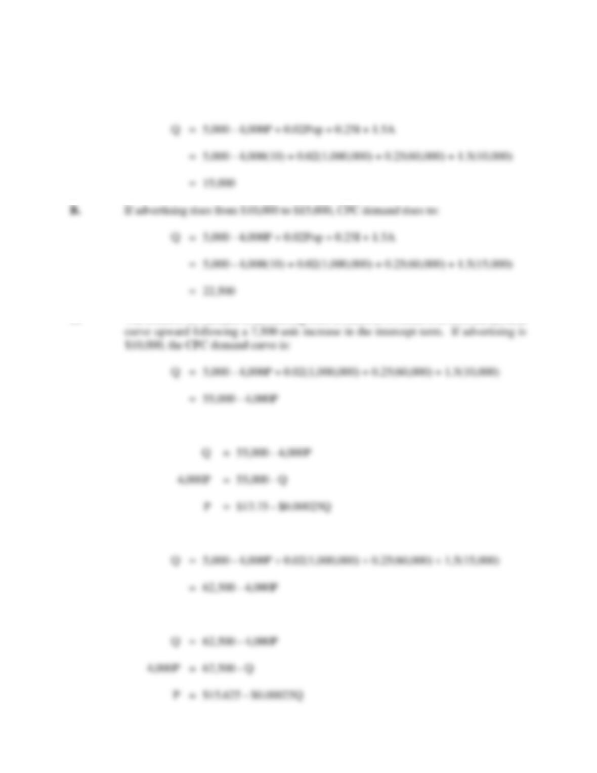
Q = 5,000 – 4,000P + 0.02Pop + 0.25I + 1.5A,
where Q is quantity, P is price ($), Pop is population, I is disposable income per
household ($), and A is advertising expenditures ($).
A. Determine the demand faced by CPC in a typical market in which P = $10, Pop =
1,000,000 persons, I = $60,000, and A = $10,000.
B. Calculate the level of demand if CPC increases annual advertising expenditures
from $10,000 to $15,000.
C. Calculate the demand curves faced by CPC in parts A and B.
P3.5 SOLUTION
Demand and Supply 61
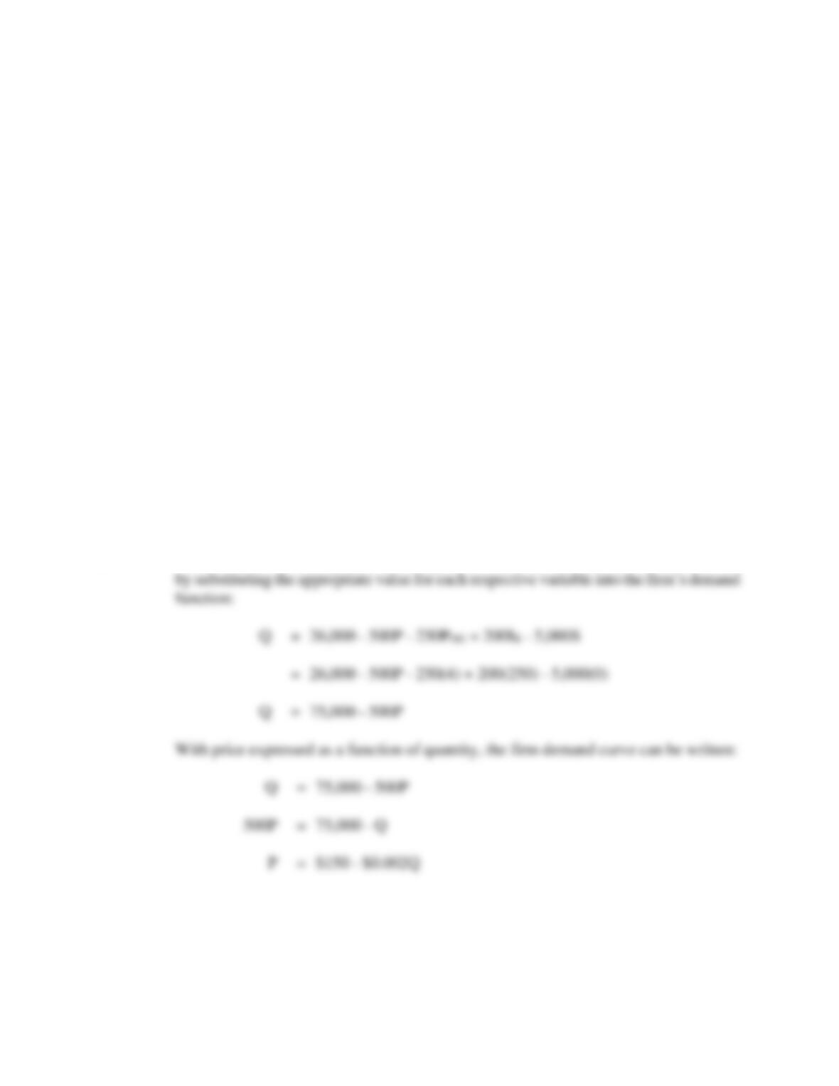
C. The effect of an increase in advertising from $10,000 to $15,000 is to shift the demand
Then, price as a function of quantity is:
If advertising is $15,000, the CPC demand curve is
Then, price as a function of quantity is:
62 Chapter 3
P3.6 Demand Curves. The Eastern Shuttle, Inc., is a regional airline providing shuttle
service between New York and Washington, D.C. An analysis of the monthly demand for
service has revealed the following demand relation:
Q = 26,000 – 500P – 250POG + 200IB – 5,000S,
where Q is quantity measured by the number of passengers per month, P is price ($),
POG is a regional price index for other consumer goods (1967 = 1.00), IB is an index of
business activity, and S, a binary or dummy variable, equals 1 in summer months and 0
otherwise.
A. Determine the demand curve facing the airline during the winter month of January
if POG = 4 and IB = 250.
B. Determine the demand curve facing the airline, quantity demanded, and total
revenues during the summer month of July if P = $100 and all other price-related
and business activity variables are as specified previously.
P3.6 SOLUTION
A. The demand curve facing Eastern during the winter month of January can be calculated