61
LECTURE SUPPLEMENT
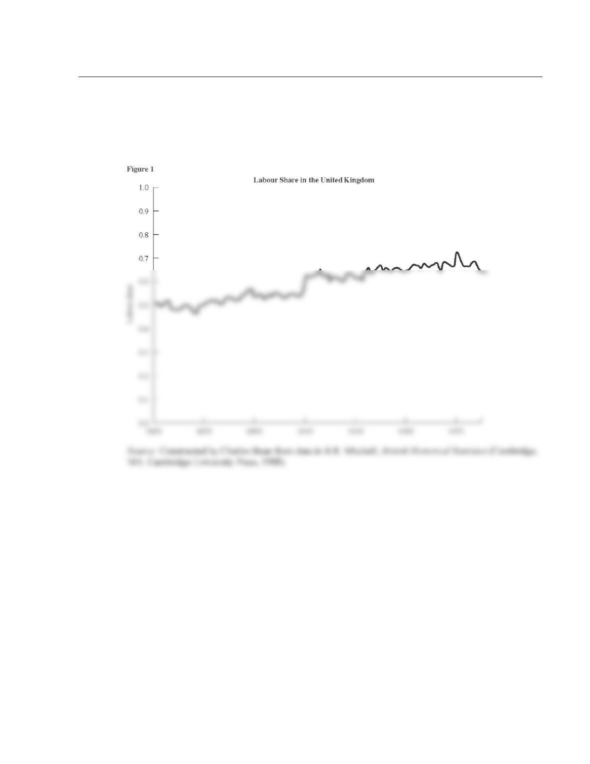
3-3 Labor’s Share of Output in the United Kingdom
Figure 3–5 in the textbook reveals that the division of U.S. output between capital and labor has been
roughly constant for the last 60 years, suggesting that the Cobb–Douglas production function is a useful
approximation. This stylized fact can be observed in other countries as well: Figure 1 graphs labor’s share
of output in the United Kingdom over the last century and a half.
62
ADDITIONAL CASE STUDY
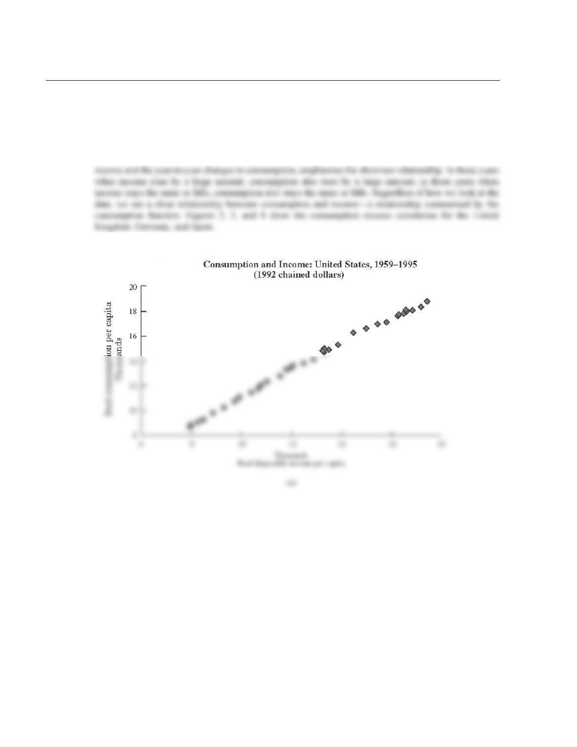
3-4 The Consumption Function
It is easy to find the consumption function in the data. Figures 1A and 1B use annual data from the
national income accounts on consumption per person and disposable income per person to illustrate the
U.S. consumption function in two different ways. Figure 1A, a scatterplot of the level of income and the
level of consumption, emphasizes the long–run relationship between these two variables. As income has
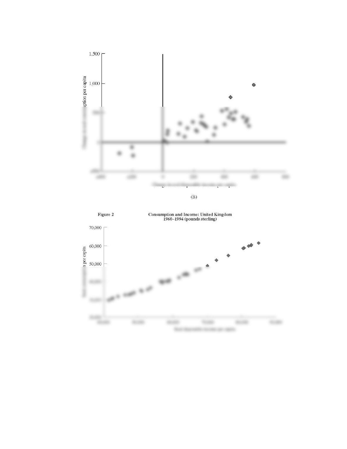
risen over time, so has consumption. Figure 1B, a scatterplot of the year–to–year changes in disposable
Figure 1a
63
Figure 1b Change in Consumption and Income: United States, 1959–1995
(1992 chained dollars)
65
LECTURE SUPPLEMENT
3-5 Economists’ Terminology
Like all sciences, economics has a well–developed terminology, or jargon. Such a language is important
because it allows economists to talk precisely about the economy and to avoid ambiguity. But this
terminology presents pitfalls for the uninitiated, since economists have an annoying habit of taking terms
that are used in everyday speech and giving them a precise meaning that may not exactly match their
everyday meanings. We consider some examples here.
Saving and Investment
In everyday speech, people use the term “investment” to refer to any purchase of an asset, such as stocks
and bonds, works of art, old or new housing, and the like. Macroeconomists usually use the term much
more precisely to refer only to certain purchases of newly produced final goods and services. If a firm
Money and Income
In everyday speech, a rich individual might be described as having a great deal of money. To the
economist, however, money is not a synonym for income or wealth. Money is the name given to a
particular asset or set of assets used for transactions. The detailed definition of money is discussed in
Profit
As discussed in Chapter 3, economists distinguish between economic profit and accounting profit. Euler’s
theorem tells us that a constant–returns–to–scale production function will imply that economic profit is zero
if factors are paid their marginal products. The idea that economists conclude that firms don’t make any
profit may seem baffling. Again, this arises because economists’ use of the term “profit” differs from the
everyday use of the term. What is normally counted as profit by a firm, the economist thinks of as a
payment to a factor of production.
66
Real and Nominal Variables
One of the most important distinctions in macroeconomics, and one that recurs throughout the textbook, is
that between real and nominal variables. The distinction is actually very simple; acquiring the habit of
Stocks Versus Flows
Economists distinguish between variables know as “stocks” and variables known as “flows.” Stocks are
measured at a point in time, whereas flows are measured over time. In the loanable funds model, saving is
67
ADDITIONAL CASE STUDY
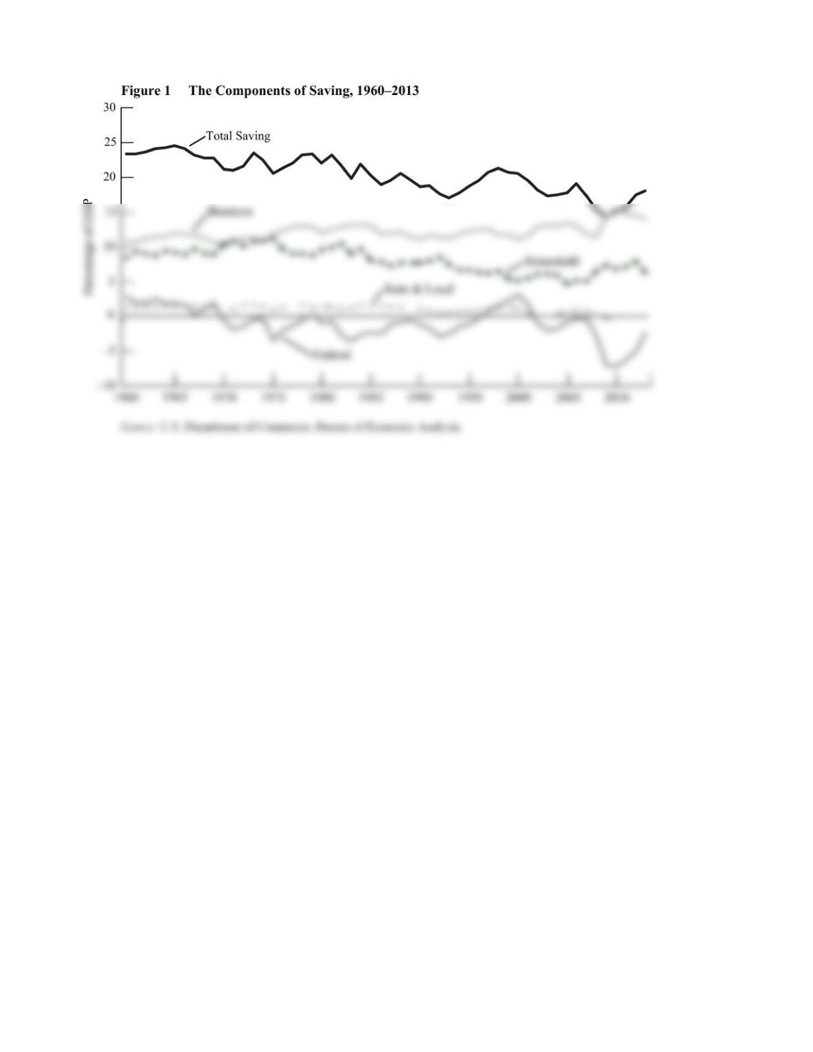
3-6 Public and Private Saving
The classical model of Chapter 3 discusses equilibrium in terms of the equality of investment and national
saving. In interpreting this model, it is crucial to remember that national saving includes both private
saving and the saving of the government. Private saving can in turn be subdivided into personal saving—
the saving of individuals—and business saving, or saving by corporations. Public or government saving
make it consistent with the manner in which private investment is calculated. Business expenditures on
equipment and structures are considered investment. Prior to the 1996 revision these expenditures, if
undertaken by the government, were considered government consumption expenditures. Thus, a new
office building purchased by the private sector would increase investment, whereas the same building if
purchased by the government would not increase investment. Now, expenditures on equipment and
68
69
ADDITIONAL CASE STUDY
3-7 Wars and Interest Rates
Wars provide a good illustration of our theory, since government expenditures usually increase greatly in
wartime. Also, wars are occasions when we can be reasonably confident that changes in government
spending are really exogenous. Often, governments’ fiscal policies may actually be responses to the state
of the economy. Between the mid–eighteenth century and the early twentieth century, the United Kingdom
was involved in a number of wars, during each of which military spending rose. As predicted by the
model, interest rates were also high at those times.
Are there other explanations for the observed correlation (in British data) between government
spending in wartime and interest rates? Robert Barro discusses two issues in his Journal of Monetary
70
LECTURE SUPPLEMENT
3-8 A First Look at Nominal and Real Interest Rates
The text describes how investment depends on the real interest rate—the rate adjusted for inflation—and
simply states that it represents the true cost of borrowing, putting aside for now the question of exactly
how real interest rates are measured. As we will see in Chapter 17, the appropriate real interest rate for
investment decisions is the ex ante or expected real interest rate, which is equal to the nominal rate minus
Some observers point to this pattern of higher ex post real interest rates in the 1980s as evidence that
the shift toward large budget deficits fireduction in government saving) during the Reagan administration
had the effect of raising the real interest rate. Such a rise is what the simple classical model described in
this chapter predicts following a decline in government saving. Others, however, argue that the ex ante
real interest rate did not follow the pattern of the ex post real interest rate because people expected the high
recovery that followed. Although inflation fell somewhat during these years, it remained above zero.
With the nominal interest rate close to zero and inflation positive, the real interest dropped below zero
from 2009 through 2013.

Table 1 Nominal and Real Interest Rates, 1962–2013 (percent)
Year
One–Year
Treasury Rate
Annual Rate
of Inflation
Real Interest
Rate
Decadal
Average
1962
3.1
1.3
1.8
1963
3.4
1.3
2.1
1964
3.9
1.6
2.3
1965
4.2
2.9
1.3
1966
5.2
3.1
2.1
1967
4.9
4.2
0.7
1968
5.7
5.5
0.2
1969
7.1
5.7
1.4
1970
6.9
4.4
2.5
1.6
1971
4.9
3.2
1.7
1972
5.0
6.2
–1.3
1973
7.3
11.0
–3.7
1974
8.2
9.1
–0.9
1975
6.8
5.8
1.0
1976
5.9
6.5
–0.6
1977
6.1
7.6
–1.5
1978
8.3
11.3
–3.0
1979
10.7
13.5
–2.9
1980
12.0
10.3
1.7
–0.9
1981
14.8
6.2
8.6
1982
12.3
3.2
9.1
1983
9.6
4.3
5.3
1984
10.9
3.6
7.3
1985
8.4
1.9
6.5
1986
6.5
3.6
2.9
1987
6.8
4.1
2.7
1988
7.7
4.8
2.9
1989
8.5
5.4
3.1
1990
7.9
4.2
3.7
5.2
1991
5.9
3.0
2.9
1992
3.9
3.0
0.9
1993
3.4
2.6
0.8
1994
5.3
2.8
2.5
1995
5.9
3.0
2.9
1996
5.5
2.3
3.2
1997
5.6
1.6
4.0
1998
5.1
2.2
2.9
1999
5.1
3.4
1.7
2000
6.1
2.8
3.3
2.5
2001
3.5
1.6
1.9
2002
2.0
2.3
–0.3
2003
1.2
2.7
–1.5
2004
1.9
3.4
–1.5
2005
3.6
3.2
0.4
2006
4.9
2.8
2.1
2007
4.5
3.8
0.7
2008
1.8
–0.4
2.2
(Continued on next page)

Table 1 Nominal and Real Interest Rates, 1962–2013 (percent) (Continued)
Year
One–Year
Treasury Rate
Annual Rate
of Inflation
Real Interest
Rate
Decadal
Average
2009
0.5
1.6
–1.1
2010
0.3
3.2
–2.9
2011
0.2
2.1
–1.9
2012
0.2
1.5
–1.3
2013
0.1
1.6
–1.5
–1.6
Note: The interest rate is the one–year constant maturity Treasury yield. Inflation is annual percent change in the consumer price