Basic Econometrics, Gujarati and Porter
17
CHAPTER 3:
TWO-VARIABLE REGRESSION MODEL:
THE PROBLEM OF ESTIMATION
3.1 (1) Y
i
=
1 2
i i
X u
β β
+ +
. Therefore,
E(Y
i
i
X
) = E[(
1
β
+
2
i
X
β
+ u
i
)
i
X
]
i
i
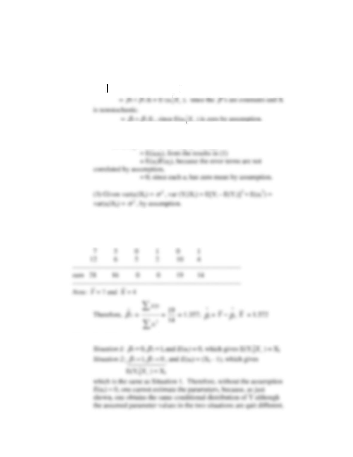
(2) Given cov(u
i
u
j
) = 0 for
∀
for all i,j (i
≠
j), then
cov(Y
i
Y
j
) = E{[Y
i
– E(Y
i
)][Y
j
– E(Y
j
)]}
3.2 Y
i
X
i
y
i
x
i
x
i
y
i
x
i2
4 1 -3 -3 9 9
5 4 -2 0 0 0
3.3
The PRF is: Y
i
=
1 2
i i
X u
β β
+ +
18
3.4
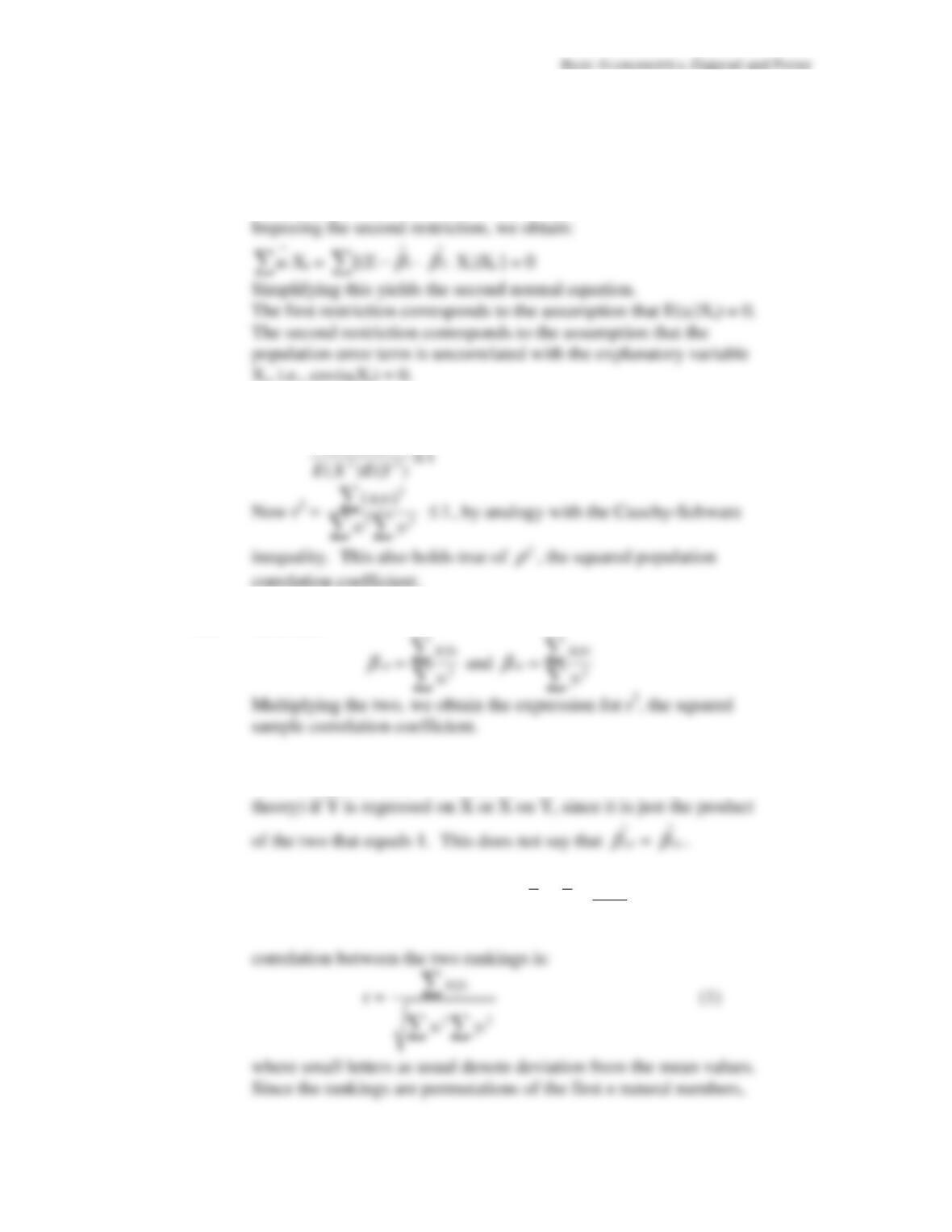
Imposing the first restriction, we obtain:
i
u
∧
∑
=
∑
(Y
i
–
1
β
∧
–
2
β
∧
X
i
) = 0
Simplifying this yields the first normal equation.
i
i
i
3.5
From the Cauchy-Schwarz inequality it follows that:
2
( )
E XY
3.6
Note that:
3.7
Even though
yx
β
∧
.
xy
β
∧
=1, it may still matter (for causality and
3.8
The means of the two-variables are:
1
2
n
Y X
+
= = and the
Basic Econometrics, Gujarati and Porter
19
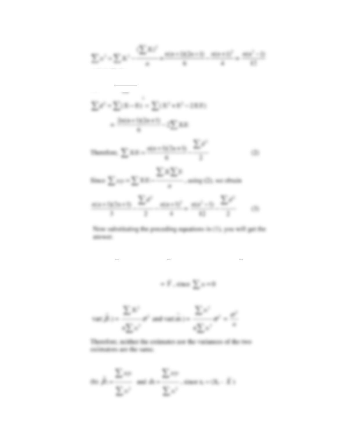
and similarly,
2
2
( 1)
i
n n
y
−
=
∑
, Then
3.9
(a)
1
β
∧
=
2
Y
β
∧
−
X
i
and
1
α
∧
=
2
Y
β
∧
−
x
−
[Note: x
i
= (X
i
–
X
)]
Basic Econometrics, Gujarati and Porter
20
3.10
Since
0
i i
x y
= =
∑ ∑
, that is, the sum of the deviations from mean
value is always zero,
x
−
=
y
−
= 0 are also zero. Therefore,
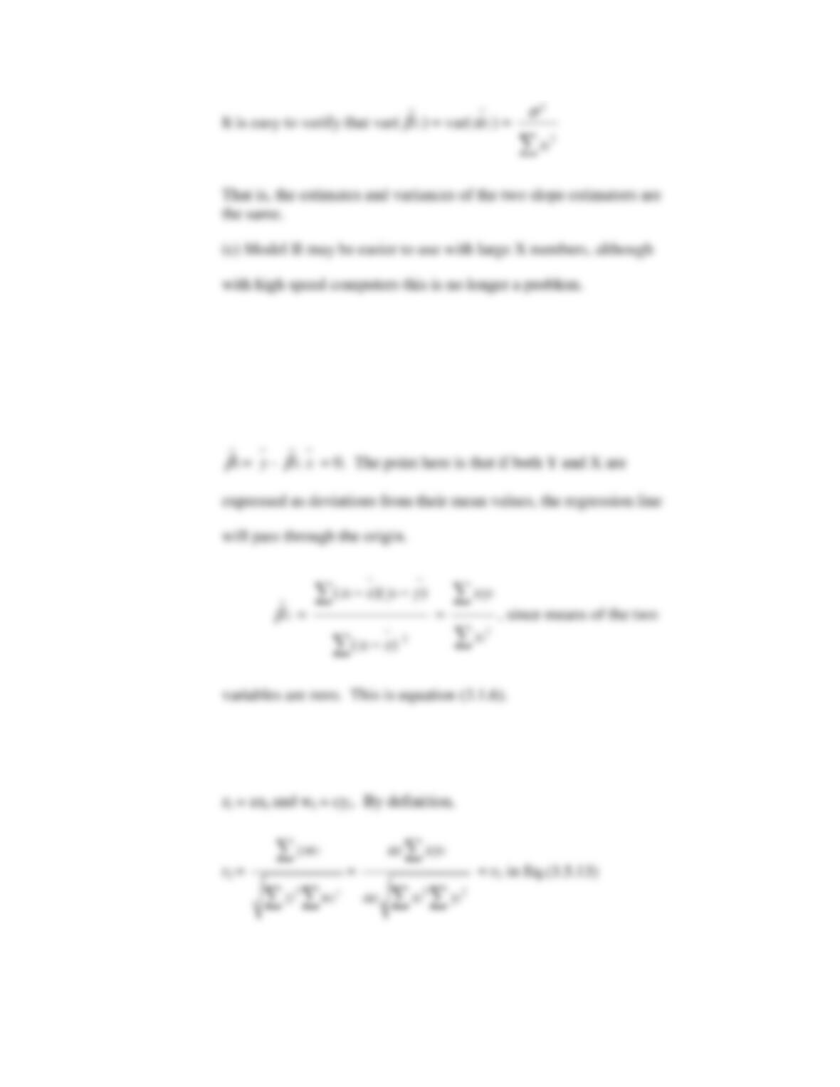
3.11
Let Z
i
= aX
i
+ b and W
i
= cYi + d. In deviation form, these become:
3.12
(a) True. Let a and c equal -1 and b and d equal 0 in Question 3.11.
Basic Econometrics, Gujarati and Porter
21
3.13
Let Z = X
1
+ X
2
and W = X
2
and X
3
. In deviation form, we can write
these as z = x
1
+ x
2
and w = x
2
+ x
3
. By definition the correlation
between Z and W is:
3.14 The residuals and fitted values of Y will not change. Let
Y
i
=
1 2
i i
X u
β β
+
+
and Y
i
=
1 2
i i
Z u
α α
+ +
, where Z = 2X
Using the deviation form, we know that
Basic Econometrics, Gujarati and Porter
22
3.15 By definition,
2
ˆ
( )
i i
y y
∑
2
ˆ ˆ ˆ
( )( )
i i i
y u y
+
∑
2
ˆ
i
y
∑
i
i
coefficient will be one and the intercept zero. But a formal proof can
proceed as follows:
3.17
Write the sample regression as:
1
ˆ
ˆ
i i
Y u
β
= +
. By LS principle, we
Basic Econometrics, Gujarati and Porter
23
with the only unknown parameter and set the resulting expression to
zero, to obtain:
Empirical Exercises
3.18
Taking the difference between the two ranks, we obtain:
d
-2 1 -1 3 0 -1 -1 -2 1 2
Therefore, Spearman’s rank correlation coefficient is
3.19
(a) The slope value of 2.250 suggests that over the period 1985-2005,
Basic Econometrics, Gujarati and Porter
24
3.20
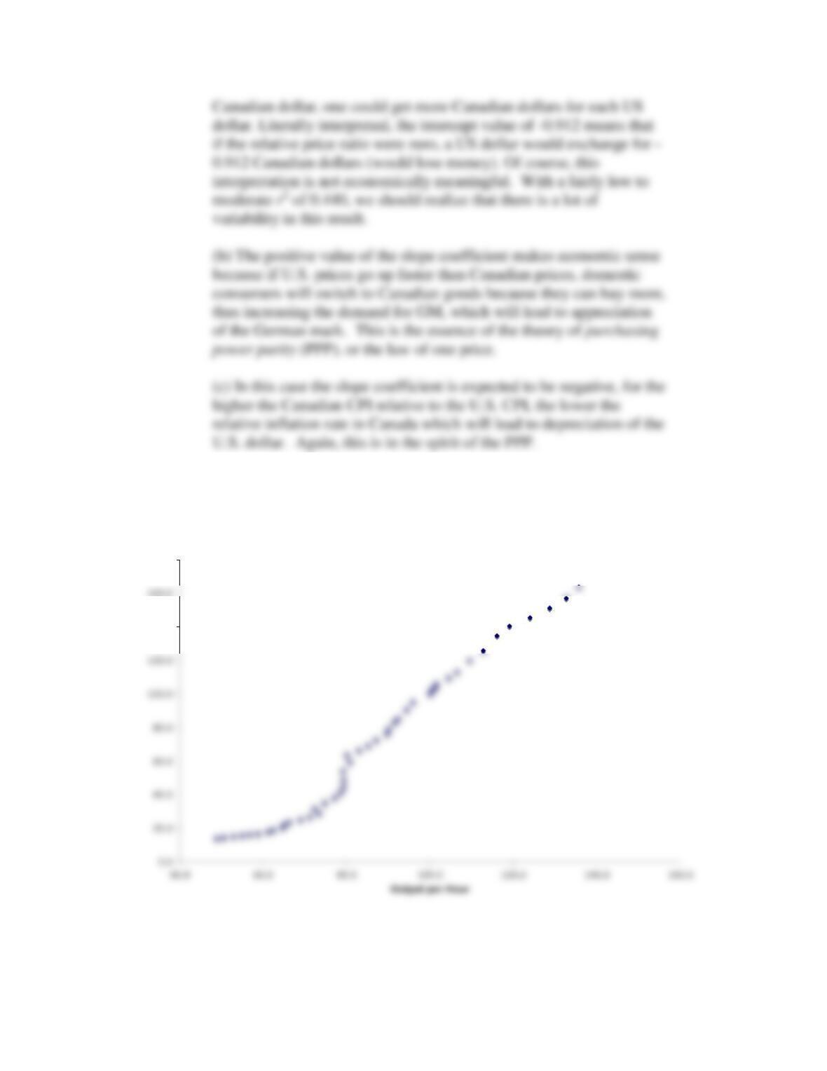
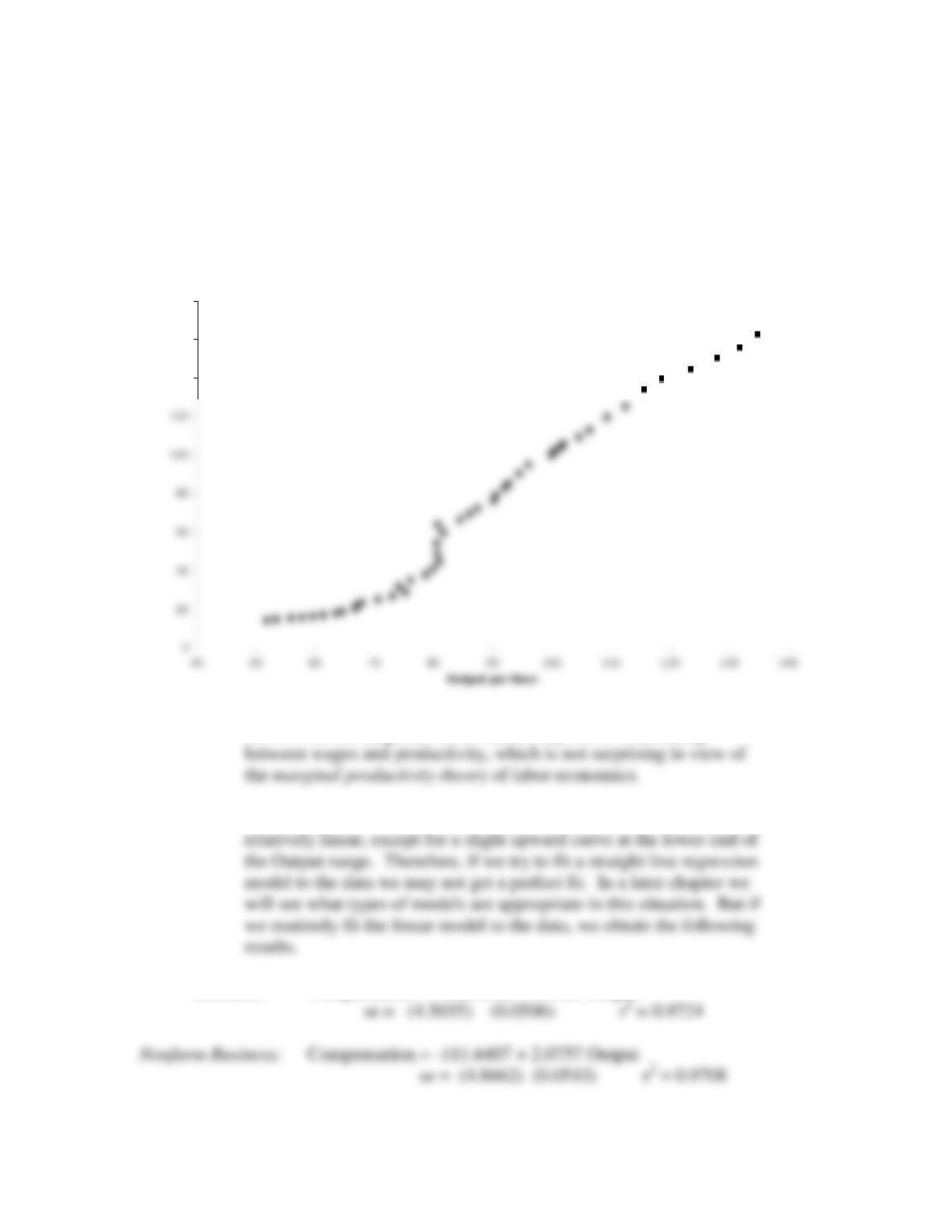
(a) The scattergrams are as follows:
Business Sector: Compensation vs Output
140.0
180.0
Basic Econometrics, Gujarati and Porter
25
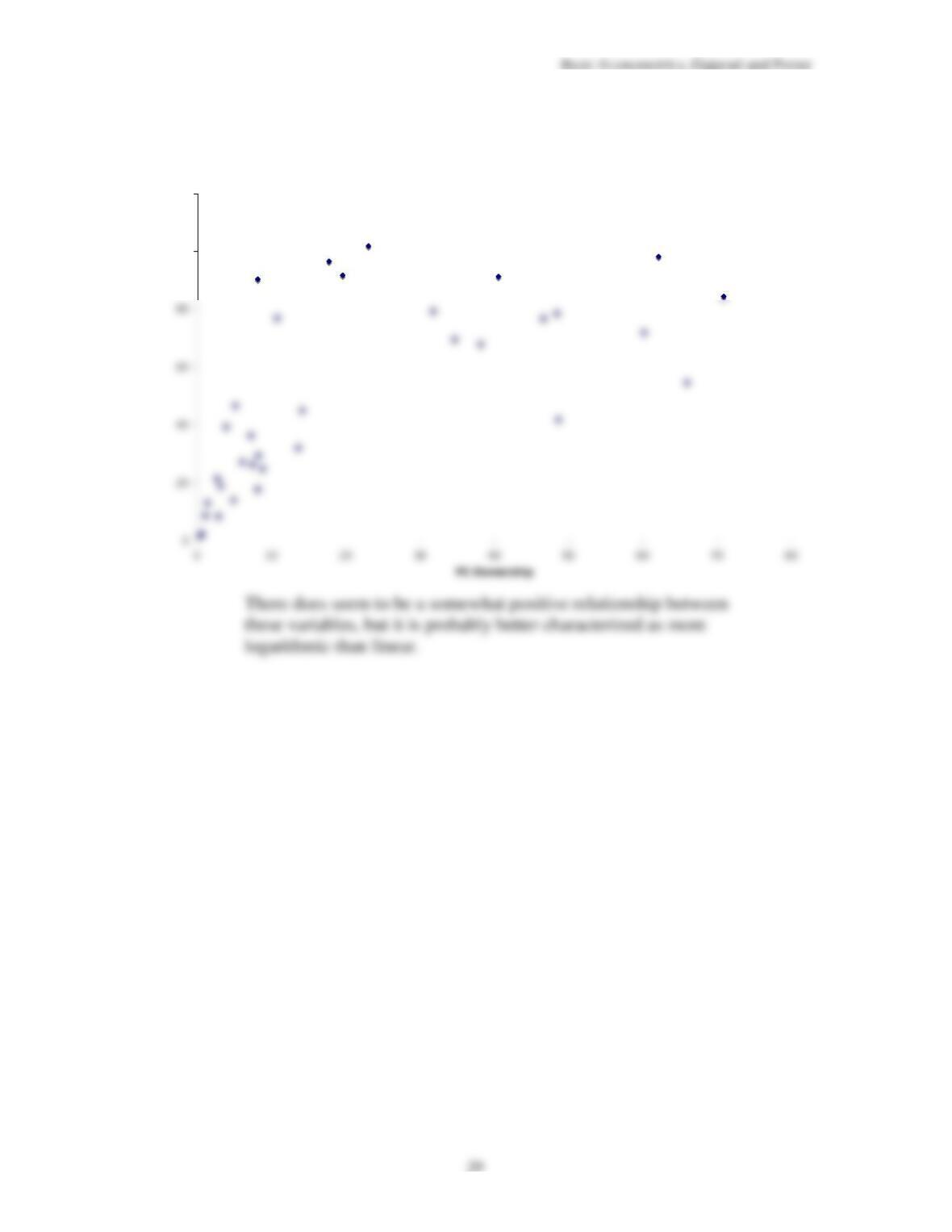
(b) As both the diagrams show, there is a positive relationship
(c) As the preceding figures show, the relationship between wages is
Business
: Compensation = -102.3662 + 1.9924 Output
Nonfarm Business Sector: Compensation vs Output
140
160
180
Basic Econometrics, Gujarati and Porter
26
3.21
i
Y
∑
i
X
∑
i i
X Y
∑
2
i
X
∑
2
i
Y
∑
3.22 (
a)
(b) If the hypothesis were true, we would expect
2
1
β
≥
.
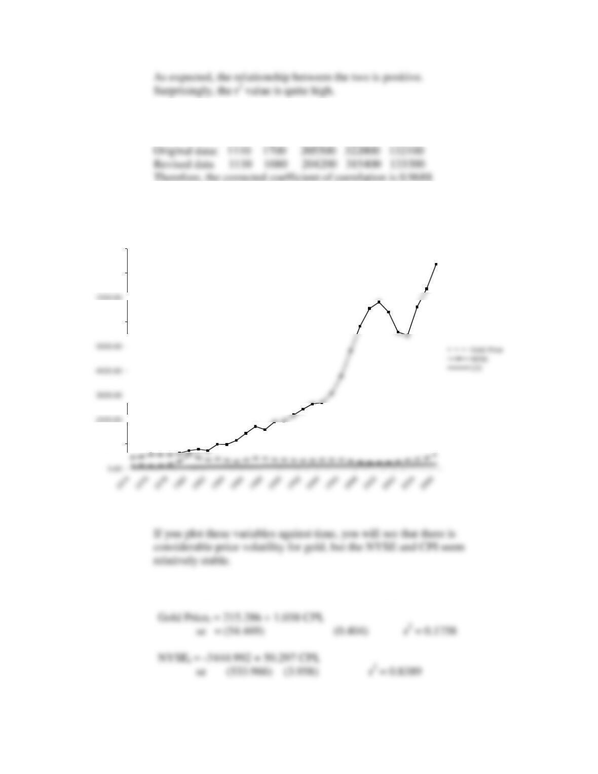
Gold Prices, CPI, and the NYSE Index Over Time
1000.00
6000.00
8000.00
9000.00
27
3.23
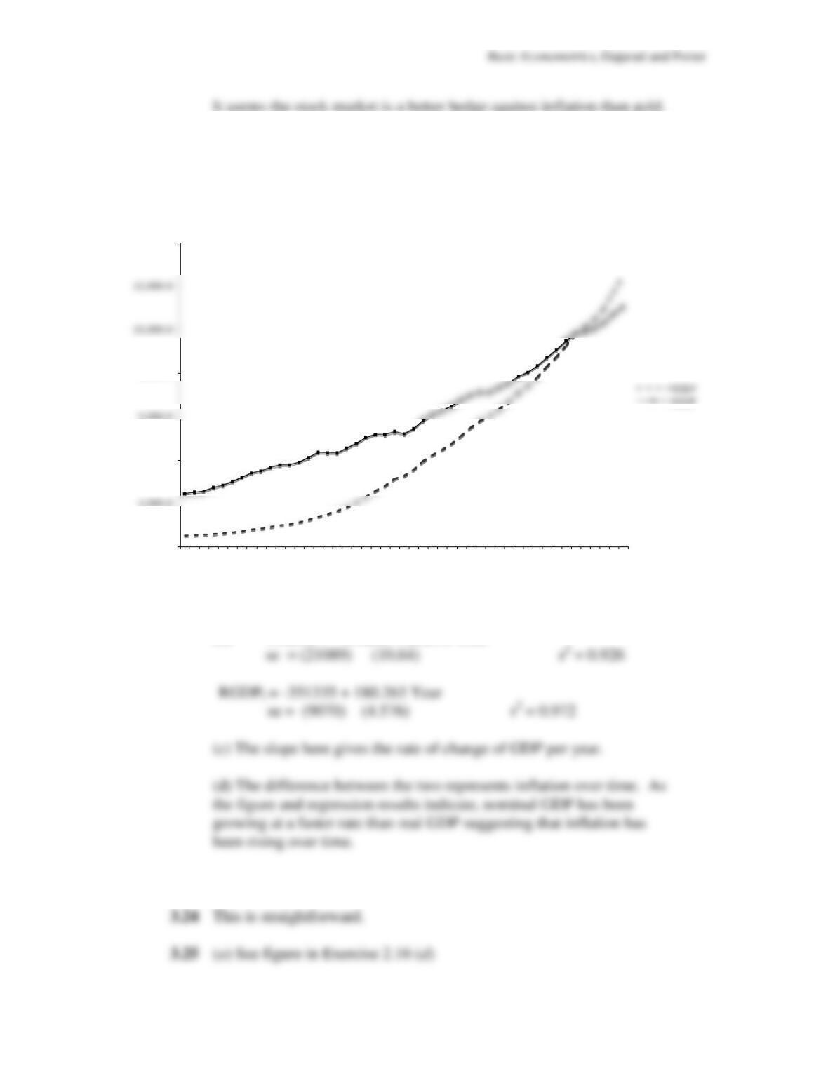
(a) The plot is as follows, where NGDP and RGDP are nominal and real
GDP.
(b) NGDP
t
= – 496268 + 252.58 Year
NGDP and RGDP Over Time
0.0
4,000.0
8,000.0
14,000.0
1959
1961
1963
1965
1967
1969
1971
1973
1975
1977
1979
1981
1983
1985
1987
1989
1991
1993
1995
1997
1999
2001
2003
2005
Basic Econometrics, Gujarati and Porter
(
b
) The regression results are:
(
c
) As pointed out in the text, a statistical relationship, however
3.26
The regression results are:
ö
Y
= −
257.02
+
1.416
X
3.28
Cell Phone Subscribers vs PC Ownership
100
120