Questions for Review
1. The factors of production and the production technology determine the amount of out-
put an economy can produce. The factors of production are the inputs used to produce
2. When a firm decides how much of a factor of production to hire or demand, it considers how
this decision affects profits. For example, hiring an extra unit of labor increases output and
therefore increases revenue; the firm compares this additional revenue to the additional
cost from the higher wage bill. The additional revenue the firm receives depends on the
marginal product of labor (MPL) and the price of the good produced (P). An additional unit
3. A production function has constant returns to scale if an equal percentage increase in
all factors of production causes an increase in output of the same percentage. For exam-
ple, if a firm increases its use of capital and labor by 50 percent, and output increases
by 50 percent, then the production function has constant returns to scale.
If the production function has constant returns to scale, then total income (or
equivalently, total output) in an economy of competitive profit-maximizing firms is
divided between the return to labor, MPL ×L, and the return to capital, MPK ×K. That
is, under constant returns to scale, economic profit is zero.
11
CHAPTER 3National Income: Where It Comes From
and Where It Goes
6. Government purchases are a measure of the dollar value of goods and services pur-
chased directly by the government. For example, the government buys missiles and
7. Consumption, investment, and government purchases determine demand for the econo-
my’s output, whereas the factors of production and the production function determine
the supply of output. The real interest rate adjusts to ensure that the demand for the
economy’s goods equals the supply. At the equilibrium interest rate, the demand for
goods and services equals the supply.
8. When the government increases taxes, disposable income falls, and therefore consumption
falls as well. The decrease in consumption equals the amount that taxes increase multi-
plied by the marginal propensity to consume (MPC). The higher the MPC is, the greater is
Problems and Applications
1. a. According to the neoclassical theory of distribution, the real wage equals the mar-
ginal product of labor. Because of diminishing returns to labor, an increase in the
labor force causes the marginal product of labor to fall. Hence, the real wage falls.
2. A production function has decreasing returns to scale if an equal percentage increase in
all factors of production leads to a smaller percentage increase in output. For example,
if we double the amounts of capital and labor, and output less than doubles, then the
production function has decreasing returns to scale. This may happen if there is a fixed
factor such as land in the production function, and this fixed factor becomes scarce as
the economy grows larger.
3. a. A Cobb–Douglas production function has the form Y= AKαL1 – α. The text showed
that the marginal products for the Cobb–Douglas production function are:
MPL = (1 – α)Y/L.
MPK = αY/K.
12 Answers to Textbook Questions and Problems
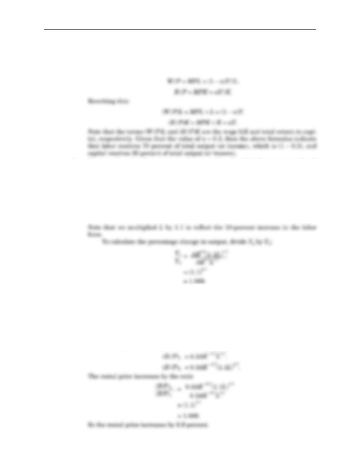
Competitive profit-maximizing firms hire labor until its marginal product
equals the real wage, and hire capital until its marginal product equals the real
rental rate. Using these facts and the above marginal products for the
Cobb–Douglas production function, we find:
b. To determine what happens to total output when the labor force increases by 10
percent, consider the formula for the Cobb–Douglas production function:
Y= AKαL1 – α.
Let Y1equal the initial value of output and Y2equal final output. We know that
α= 0.3. We also know that labor Lincreases by 10 percent:
Y1= AK0.3L0.7.
Y2= AK0.3(1.1L)0.7.
That is, output increases by 6.9 percent.
To determine how the increase in the labor force affects the rental price of
capital, consider the formula for the real rental price of capital R/P:
R/P = MPK = αAKα– 1L1 – α.
We know that α= 0.3. We also know that labor (L) increases by 10 percent. Let
(R/P)1equal the initial value of the rental price of capital, and (R/P)2equal the
final rental price of capital after the labor force increases by 10 percent. To find
(R/P)2, multiply Lby 1.1 to reflect the 10-percent increase in the labor force:
Chapter 3 National Income: Where It Comes From and Where It Goes 13
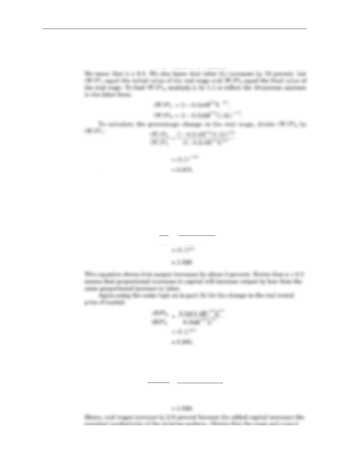
To determine how the increase in the labor force affects the real wage, con-
sider the formula for the real wage W/P:
W/P = MPL = (1 – α)AKαL– α.
That is, the real wage falls by 2.8 percent.
c. We can use the same logic as in part (b) to set
Y1= AK0.3L0.7.
Y2= A(1.1K)0.3L0.7.
Therefore, we have:
=
The real rental price of capital falls by 6.5 percent because there are diminishing
returns to capital; that is, when capital increases, its marginal product falls.
Finally, the change in the real wage is:
=
(1.1)0.3
marginal productivity of the existing workers. (Notice that the wage and output
14 Answers to Textbook Questions and Problems
A(1.1K)0.3L0.7
AK0.3L0.7
Y2
Y1
0.7A(1.1K)0.3L–0.3
0.7AK 0.3L–0.3
(W/P)2
(W/P)1
have both increased by the same amount, leaving the labor share unchanged—a
feature of Cobb–Douglas technologies.)
d. Using the same formula, we find that the change in output is:
=
= 1.1.
4. Labor income is defined as
Labor’s share of income is defined as
5. a. According to the neoclassical theory, technical progress that increases the margin-
al product of farmers causes their real wage to rise.
b. The real wage for farmers is measured as units of farm output per worker. The
real wage is
W
/
P
F
, and this is equal to ($/worker)/($/unit of farm output).
c. If the marginal productivity of barbers is unchanged, then their real wage is
unchanged.
d. The real wage for barbers is measured as haircuts per worker. The real wage is
W/P
B
, and this is equal to ($/worker)/($/haircut).
Chapter 3 National Income: Where It Comes From and Where It Goes 15
(1.1A)K0.3L0.7
AK0.3L0.7
Y2
Y1
W
P
LWL
P
¥= .
6. a. The marginal product of labor MPL is found by differentiating the production
function with respect to labor:
MPL =
= K1/3H1/3L–2/3.
An increase in human capital will decrease the marginal product of human capital
because there are diminishing returns.
c. The labor share of output is the proportion of output that goes to labor. The total
amount of output that goes to labor is the real wage (which, under perfect compe-
tition, equals the marginal product of labor) times the quantity of labor. This
quantity is divided by the total amount of output to compute the labor share:
so labor gets one-third of the output, and human capital gets one-third of the out-
put. Since workers own their human capital (we hope!), it will appear that labor
gets two-thirds of output.
d. The ratio of the skilled wage to the unskilled wage is:
e. If more college scholarships increase H, then it does lead to a more egalitarian
society. The policy lowers the returns to education, decreasing the gap between
the wages of more and less educated workers. More importantly, the policy even
raises the absolute wage of unskilled workers because their marginal product
rises when the number of skilled workers rises.
3
dY
dL
1
3
7. The effect of a government tax increase of $100 billion on (a) public saving, (b) private
saving, and (c) national saving can be analyzed by using the following relationships:
National Saving = [Private Saving] + [Public Saving]
= [Y– T– C(Y– T)] + [T– G]
= Y– C(Y– T) – G.
a. Public Saving—The tax increase causes a 1-for-1 increase in public saving. T
increases by $100 billion and, therefore, public saving increases by $100 billion.
Another way to see this is by using the third equation for national saving
expressed above, that national saving equals Y– C(Y– T) – G. The $100 billion
tax increase reduces disposable income and causes consumption to fall by $60 bil-
lion. Since neither Gnor Ychanges, national saving thus rises by $60 billion.
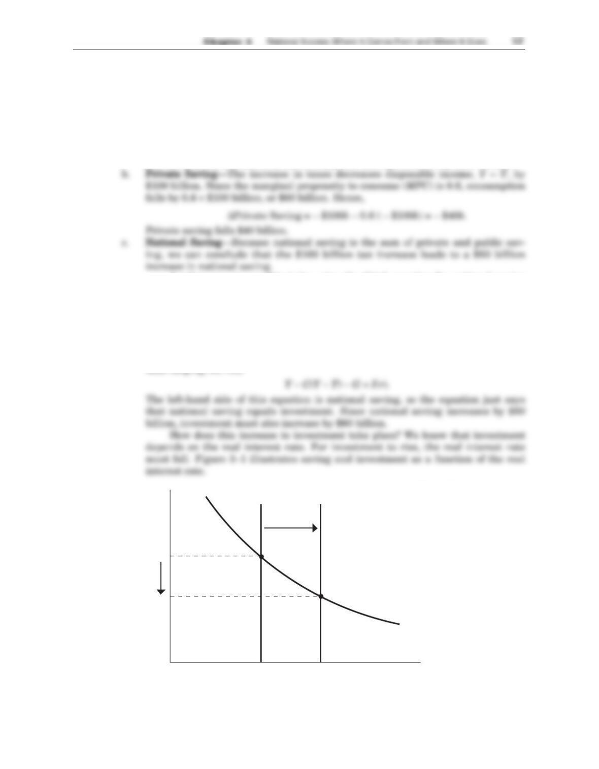
d. Investment—To determine the effect of the tax increase on investment, recall the
national accounts identity:
Y= C(Y– T) + I(r) + G.
Rearranging, we find
The tax increase causes national saving to rise, so the supply curve for loan-
able funds shifts to the right. The equilibrium real interest rate falls, and invest-
ment rises.
S1S2
I (r)
I, S
Investment, Savin
g
r1
r2
r
Real interest rate
Figure 3–1
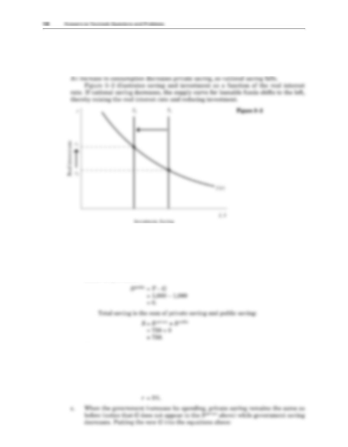
8. If consumers increase the amount that they consume today, then private saving and,
therefore, national saving will fall. We know this from the definition of national saving:
National Saving = [Private Saving] + [Public Saving]
= [Y– T– C(Y– T)] + [T– G].
9. a. Private saving is the amount of disposable income, Y – T, that is not consumed:
Sprivate = Y – T – C
= 5,000 – 1,000 – (250 + 0.75(5,000 – 1,000))
= 750.
Public saving is the amount of taxes the government has left over after it
makes its purchases:
b. The equilibrium interest rate is the value of rthat clears the market for loanable
funds. We already know that national saving is 750, so we just need to set it equal
to investment:
S= I
750 = 1,000 – 50r
Solving this equation for r, we find:
g
Sprivate = 750
d. Once again the equilibrium interest rate clears the market for loanable funds:
S= I
500 = 1,000 – 50r
Solving this equation for r, we find:
r= 10%.
10. To determine the effect on investment of an equal increase in both taxes and govern-
ment spending, consider the national income accounts identity for national saving:
National Saving = [Private Saving] + [Public Saving]
= [Y– T– C(Y– T)] + [T– G].
The above expression tells us that the impact on saving of an equal increase in T
and Gdepends on the size of the marginal propensity to consume. The closer the MPC
is to 1, the smaller is the fall in saving. For example, if the MPC equals 1, then the fall
in consumption equals the rise in government purchases, so national saving [Y– C(Y–
T) – G] is unchanged. The closer the MPC is to 0 (and therefore the larger is the
amount saved rather than spent for a one-dollar change in disposable income), the
greater is the impact on saving. Because we assume that the MPC is less than 1, we
expect that national saving falls in response to an equal increase in taxes and govern-
ment spending.
Chapter 3 National Income: Where It Comes From and Where It Goes 19
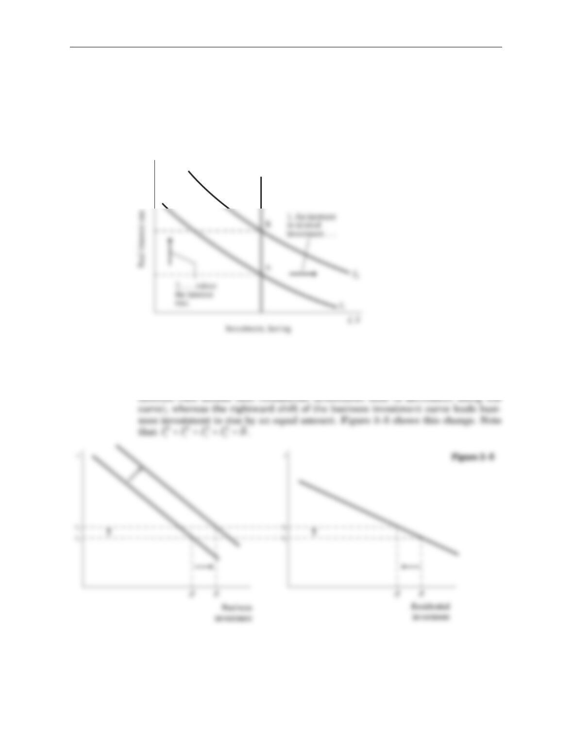
11. a. The demand curve for business investment shifts out to the right because the sub-
sidy increases the number of profitable investment opportunities for any given
interest rate. The demand curve for residential investment remains unchanged.
b. The total demand curve for investment in the economy shifts out to the right since
it represents the sum of business investment, which shifts out to the right, and
residential investment, which is unchanged. As a result the real interest rate rises
as in Figure 3–4.
c. The total quantity of investment does not change because it is constrained by the
inelastic supply of savings. The investment tax credit leads to a rise in business
investment, but an offsetting fall in residential investment. That is, the higher
12. In this chapter, we concluded that an increase in government expenditures reduces
national saving and raises the interest rate; it therefore crowds out investment by the
full amount of the increase in government expenditure. Similarly, a tax cut increases
disposable income and hence consumption; this increase in consumption translates into
a fall in national saving—again, it crowds out investment by the full amount of the
increase in consumption.
20 Answers to Textbook Questions and Problems
S
r
Figure 3–4
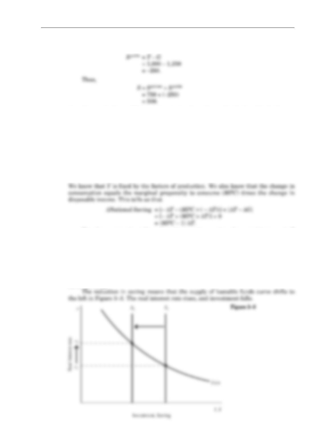
Consider what happens when government purchases increase. At any given level
of the interest rate, national saving falls by the change in government purchases, as
shown in Figure 3–7. The figure shows that if the saving function slopes upward,
investment falls by less than the amount that government purchases rises by; this hap-
pens because consumption falls and saving increases in response to the higher interest
rate. Hence, the more responsive consumption is to the interest rate, the less govern-
ment purchases crowd out investment.
Chapter 3 National Income: Where It Comes From and Where It Goes 21
S2(r)S1(r)
r
Figure 3–7

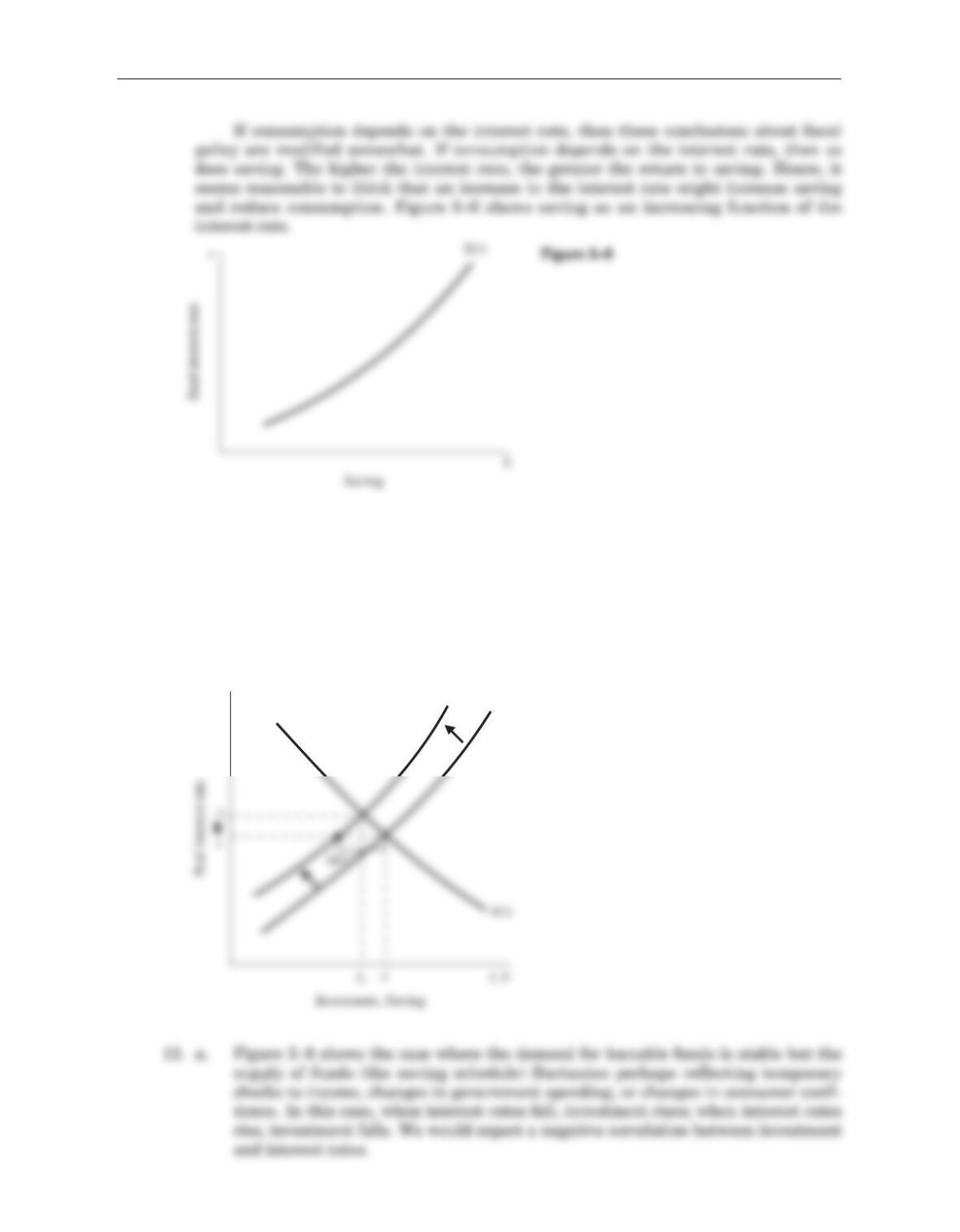
b. Figure 3-9 shows the case where the supply of loanable funds (saving) does not
respond to the interest rate. Also suppose that this curve is stable, whereas the
demand for loanable funds varies, perhaps reflecting fluctuations in firms’ expec-
tations about the marginal product of capital. We would now find a positive corre-
lation between investment and the interest rate—when demand for funds rises,
this pushes up the interest rate, so we see investment increase and the real inter-
est rate increase at the same time.
22 Answers to Textbook Questions and Problems
S2
S1
r
(r)
(r)
Figure 3–8
S(r)
r
Figure 3–9
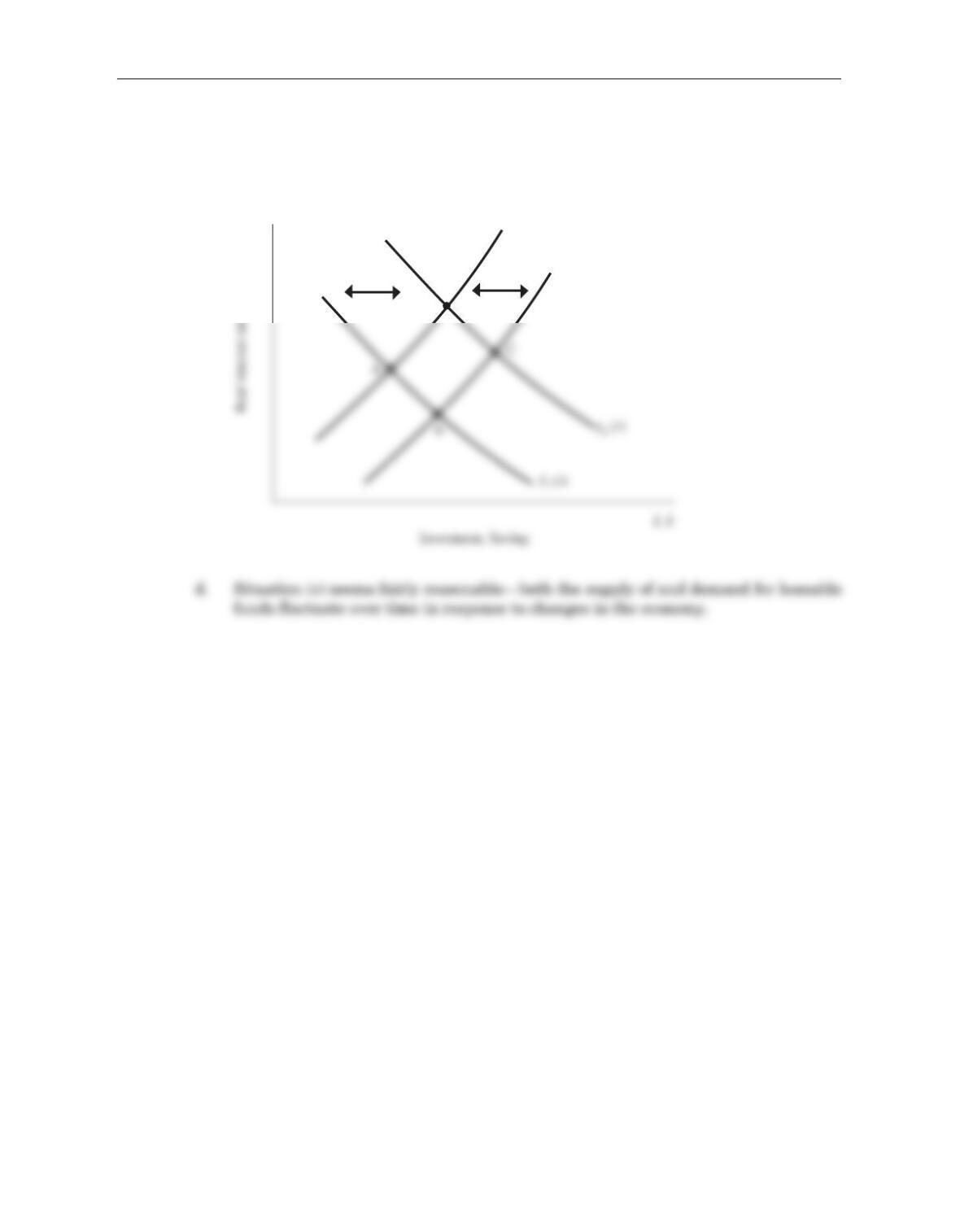
c. If both curves shift, we might generate a scatter plot as in Figure 3–10, where the
economy fluctuates among points A, B, C, and D. Depending on how often the
economy is at each of these points, we might find little clear relationship between
investment and interest rates.
Chapter 3 National Income: Where It Comes From and Where It Goes 23
r
S2(r)
S1(r)
D
Figure 3–10