
Chapter 3
Productivity, Output, and Employment
◼ Learning Objectives
I. Goals of Part 2: The Macroeconomics of Full Employment
A. Analyze factors that affect the longer-term performance of the economy
II. Goals of Chapter 3
A. Discuss production function properties and changes (Section 3.1)
B. Discuss factors that affect the demand for labor (Section 3.2)
III. Notes to Eighth Edition Users
A. We added a new box on alternative measures of the unemployment rate
between the textbook and MyEconLab

Chapter 3 Productivity, Output, and Employment 35
◼ Teaching Notes
I. How Much Does the Economy Produce? The Production Function (Sec. 3.1)
A. Factors of production
1. Capital (K)
B. The production function
1. Y = AF(K, N) (3.1)
2. Parameter A is “total factor productivity” (the effectiveness with which capital and labor
Numerical Problem 1 gives students practice working with a production function.
3. Productivity growth calculated using production function
Data Application
An example of the sharp movements in productivity that are possible can be seen by comparing
data on productivity for 2003 to data for 2004. Employment grew about the same amount in both
b. Productivity grew rapidly in the second half of the 1990s, but grew much more slowly in
the 2000s
Policy Application
Perhaps the greatest source of uncertainty facing policymakers in the 1990s and early 2000s was
36 Abel/Bernanke/Croushore • Macroeconomics, Ninth Edition
D. The shape of the production function
1. Two main properties of production functions
2. Graph production function (Y vs. one input; hold other input and A fixed)
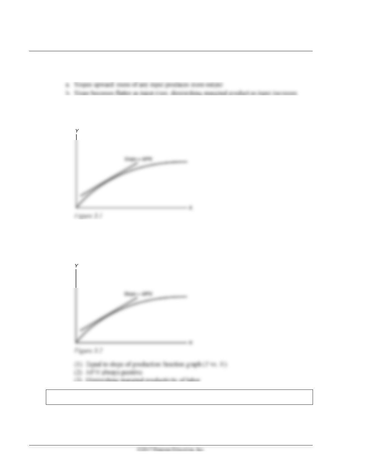
a. Marginal product of capital, MPK = Y/K (Figure 3.1; Key Diagram 1; like text
Figure 3.2)
(1) Equal to slope of production function graph (Y vs. K)
(2) MPK always positive
(3) Diminishing marginal productivity of capital—MPK—declines as K rises
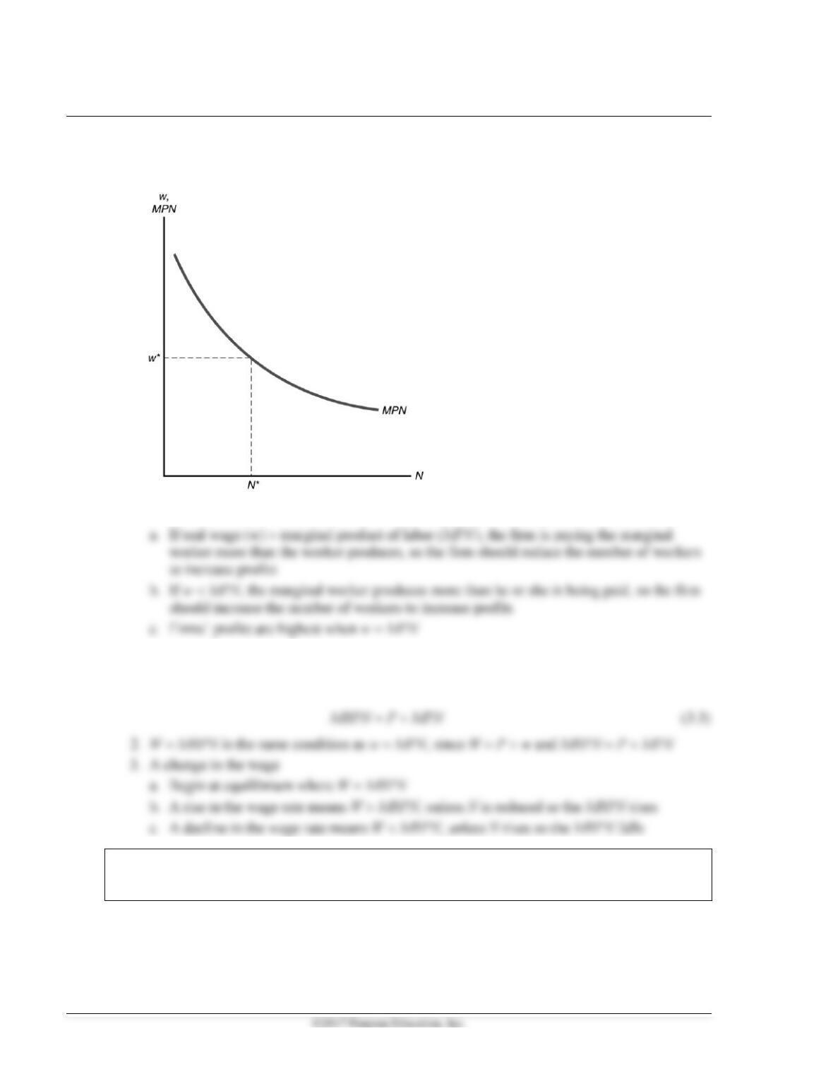
b. Marginal product of labor, MPN = Y/N (Figure 3.2; like text Figure 3.3)
(3) Diminishing marginal productivity of labor
Numerical Problem 2 gives students practice calculating the MPK and MPN.

Chapter 3 Productivity, Output, and Employment 37
E. Supply shocks
1. Supply shock = productivity shock = a change in an economy’s production function
2. Supply shocks affect the amount of output that can be produced for a given amount of inputs
Analytical Problem 1 asks students to draw production functions and show how they change
when there are supply shocks.
Theoretical Application
At this point, the instructor may wish to introduce the idea of real business cycle analysis
II. The Demand for Labor (Sec. 3.2)
A. How much labor do firms want to use?
1. Assumptions
a. Hold capital stock fixed—short-run analysis
38 Abel/Bernanke/Croushore • Macroeconomics, Ninth Edition
2. Analysis at the margin: costs and benefits of hiring one extra worker (Figure 3.4; like text
Figure 3.5)
Figure 3.4
B. The marginal product of labor and labor demand: an example
1. Example: The Clip Joint—setting the nominal wage equal to the marginal revenue product
of labor
Numerical Problem 3 sets up an example in which students calculate MPN and see what happens
when the wage rate or price of the product changes.
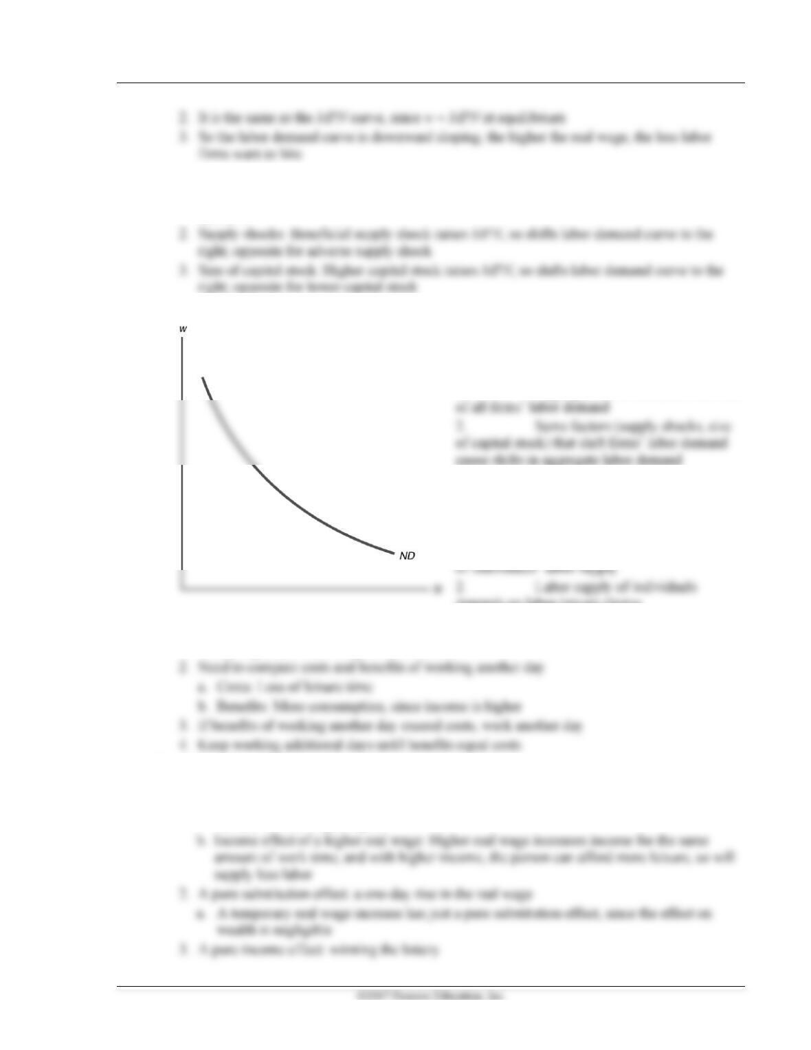
C. The marginal product of labor and the labor demand curve
1. Labor demand curve shows relationship between the real wage rate and the quantity of labor
demanded
Chapter 3 Productivity, Output, and Employment 39
D. Factors that shift the labor demand curve
1. Note: A change in the wage causes a movement along the labor demand curve, not a shift of
the curve
E. Aggregate labor demand (Figure 3.5)
Figure 3.5
1. Aggregate labor demand is the sum
III. The Supply of Labor (Sec. 3.3)
A. Supply of labor is determined by
individuals
1. Aggregate supply of labor is sum
depends on labor-leisure choice
B. The income-leisure trade-off
1. Utility depends on consumption and leisure
C. Real wages and labor supply
1. An increase in the real wage has offsetting income and substitution effects
a. Substitution effect of a higher real wage: Higher real wage encourages work, since the
reward for working is higher

40 Abel/Bernanke/Croushore • Macroeconomics, Ninth Edition
4. The substitution effect and the income effect together: a long-term increase in the real wage
a. The reward to working is greater: a substitution effect toward more work
5. Empirical evidence on real wages and labor supply
a. Overall result: Labor supply increases with a temporary rise in the real wage
b. Labor supply falls with a permanent increase in the real wage
Theoretical Application
Analytical Problem 7 examines how workers might change their labor supply if there are changes
in Social Security taxes.
D. The labor supply curve (Figure 3.6; like text Figure 3.7)
1. Increase in the current real wage should raise quantity of labor supplied

Chapter 3 Productivity, Output, and Employment 41
Theoretical Application
The field of labor economics studies the determinants of labor supply. One of the major issues in
the 1970s and early 1980s had to do with the increased participation rates of women in the labor
the recession of 2007–2009.
3. Labor supply curve slopes upward because higher wage encourages people to work more
E. Factors that shift the labor supply curve
1. Wealth: Higher wealth reduces labor supply (shifts labor supply curve to the left; text
Fig. 3.8)
Analytical problem 4 asks students to think about factors that shift an individual’s labor supply
curve.
F. Aggregate labor supply
1. Aggregate labor supply rises when current real wage rises
2. Factors increasing labor supply
a. Decrease in wealth
Data Application
A broad characterization of labor force participation rates (LFPR) is that men’s LFPR had
IV. Labor Market Equilibrium (Sec. 3.4)
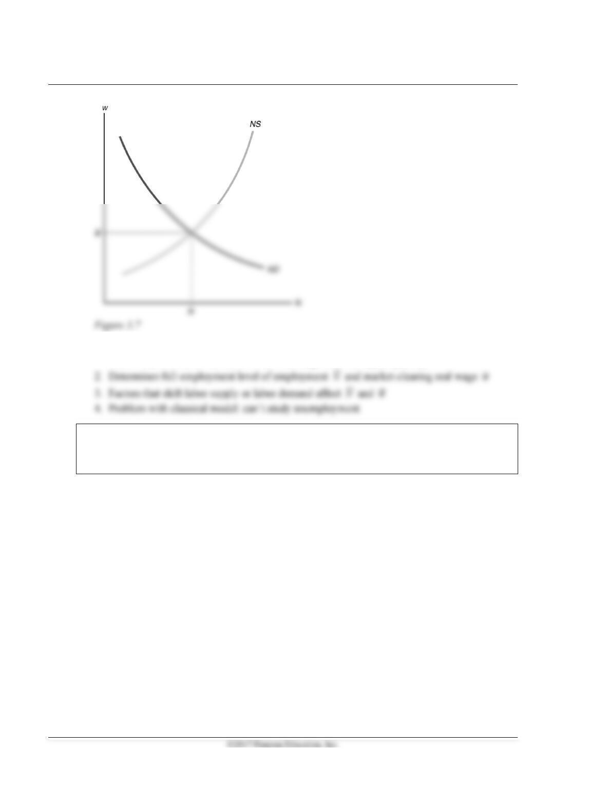
A. Equilibrium: Labor supply equals labor demand (Figure 3.7; Key Diagram 2; like text
Figure 3.9)
42 Abel/Bernanke/Croushore • Macroeconomics, Ninth Edition
1. Classical model of the labor market—real wage adjusts quickly (later, in Chapter 11, look at
other models of labor market in which real wage does not adjust quickly)
Numerical Problems 4, 5, and 6 are exercises in which students are given algebraic labor demand
and supply curves and are asked to find the equilibrium. Analytical Problems 3 and 5 are
comparative static exercises dealing with labor market equilibrium.

Chapter 3 Productivity, Output, and Employment 43
Data Application
There are, of course, many different wages in the economy; our model with just one wage is a
Data Application
Real wage growth changes substantially over time. In the 1960s, real wages grew 26%, but wage
Reserve Bank of St. Louis, variable COMPRNFB.)
Real Wage Growth by Decade (percent per decade)
1960s 26%
B. Full-employment output
1. Full-employment output = potential output =
Y
= level of output when labor market is in
equilibrium
Analytical Problem 2 asks students to show how different shocks to the economy affect full-
employment output.
Data Application
What is full-employment output? For many of our theories about macroeconomics, we need a
C. Application: output, employment, and the real wage during oil price shocks
1. Sharp oil price increases in 1973–1974, 1979–1980, 2003–2008 (text Fig. 3.11)

44 Abel/Bernanke/Croushore • Macroeconomics, Ninth Edition
4. Research result: 10% increase in price of oil reduces GDP by 0.4 percentage points
V. Unemployment (Sec. 3.5)
A. Measuring unemployment
1. Categories: employed, unemployed, not in the labor force
Data Application
The unemployment rate jumped up sharply in January 1994, not because of any true change in
the labor market, but merely because the Bureau of Labor Statistics changed the survey with
4. Participation Rate = Labor Force/Adult Population
B. Changes in employment status
1. Flows between categories (text Fig. 3.12)
2. Discouraged workers: people who have become so discouraged by lack of success at finding
a job that they stop searching
Data Application
Numerical Problems 7 and 8 are quantitative exercises using the unemployment and employment
concepts.
C. How long are people unemployed?
1. Most unemployment spells are of short duration
2. Most unemployed people on a given date are experiencing unemployment spells of long
duration

Chapter 3 Productivity, Output, and Employment 45
3. Reconciling 1 and 2—numerical example:
a. Labor force = 100; on the first day of every month, two workers become unemployed for
one month each; on the first day of every year, four workers become unemployed for one
D. Application: Unemployment Duration and the 2007–2009 Recession
1. The mean duration of unemployment always rises in recessions but in the 2007–2009 the rise
E. Why there are always unemployed people
1. Frictional unemployment
a. Search activity of firms and workers due to heterogeneity
Policy Application
Because the matching process in labor markets takes time, government policy often provides
2. Structural unemployment
a. Chronically unemployed: workers who are unemployed a large part of the time
3. The natural rate of unemployment
a.
u
= natural rate of unemployment; when output and employment are at full-employment
u
Data Application
There is much controversy about how to measure the natural rate of unemployment, as we will

46 Abel/Bernanke/Croushore • Macroeconomics, Ninth Edition
4. In touch with data and research: labor market data
a. BLS employment report
5. In touch with data and research: alternative measures of the unemployment rate
a. U-1: unemployed 15 weeks or more
b. U-2: counts job losers or persons who completed temporary jobs, so it does not
count people who have quit their jobs
Data Application
The household and establishment surveys often give conflicting results. In September 2012, the
VI. Relating Output and Unemployment: Okun’s Law (Sec. 3.6)
A. Relationship between output (relative to full-employment output) and cyclical unemployment
Data Application
What’s more closely related to output? Employment growth (from the establishment survey) or
B. (
Y
− Y)/
Y
= 2 (u −
u
) (3.5)
C. Why is the Okun’s Law coefficient 2, and not 1?
1. Other things happen when cyclical unemployment rises: Labor force falls, hours of work per

Chapter 3 Productivity, Output, and Employment 47
D. Alternative formulation if average growth rate of full-employment output is 3%:
Data Application
In 2009, the unemployment rate increased far more than expected (or, output did not decline as
much as expected) under Okun’s law. The reason was remarkably strong growth in productivity

48 Abel/Bernanke/Croushore • Macroeconomics, Ninth Edition
◼ Additional Issues for Classroom Discussion
1. Is the Unemployment Rate a Good Measure of Economic Distress?
Macroeconomists often treat the unemployment rate as the key indicator of the business cycle. But terms
2. What Else Is Important for Production?
3. As Your Wage Rises, Do You Supply More Labor? Or Less?
The textbook discusses the offsetting income and substitution effects on labor supply of an increase in the
4. Why Do Oil Price Shocks Hurt the Economy So Much?
The textbook points out that many recessions are associated with increases in oil prices. The reasons that