Economics Chapter 3 Develop a theoretical model of the macroeconomy

CHAPTER 3: PRODUCTIVITY, OUTPUT, AND EMPLOYMENT

LEARNING OBJECTIVES

I. Goals of Part 2: Long-Run Economic Performance

A. Analyze factors that affect the longer-term performance of the economy

B. Develop a theoretical model of the macroeconomy

1. Three markets

II. Goals of Chapter 3

A. Introduce the production function as the main determinant of output

1. Discuss the marginal productivity of labour and capital

2. Analyze supply shocks

B. Discuss the determinants of labour demand and supply

TEACHING NOTES

I. How Much Does the Economy Produce? The Production Function (Sec. 3.1)

A. Factors of production

1. Capital

Numerical Problem 1 gives students practice working with a production function

3. Productivity growth calculated using production function

a. Productivity moves sharply from year to year

b. Productivity growth relatively slow since 1980

Productivity, Output, and Employment 29

Data Application

Productivity in the Canadian economy can be very volatile. It tends to go down in a recession

and up during a recovery. For data on Canadian productivity (and comparisons with the

United States and between Canadian provinces) see the Centre for the Study of Living

Standards web site at www.csls.ca and search under “projects” and “data base.”

2. Graph production function (Y vs. one input; hold other input and A

fixed)

a. Marginal product of capital,

MPK = ΔY/ΔK (Fig. 3.1; Key

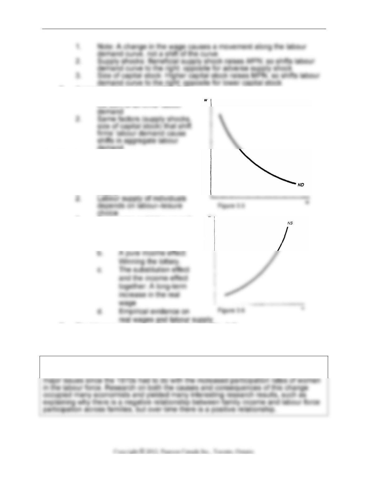
b. Marginal product of labour,

MPN = ΔY/ΔN (Fig. 3.2; like

Numerical Problem 2 gives students practice calculating the MPK and MPN.

E. Supply shocks

1. Supply shocks affect the amount of output that can be produced for a

30 Chapter 3

Data Application

Why haven’t computers increased productivity? We’re living in the information age, in

which many chores that used to take hours of labour can be done in seconds, such as

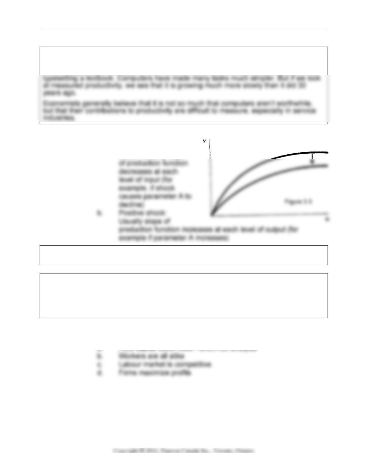
4. Supply shocks shift the graph of the production function (Fig. 3.3; like

text Fig. 3.4)

a. Negative (adverse)

shock: Usually slope

Analytical Problem 1 asks students to draw production functions and show how they

change when there are supply shocks.

Theoretical Application

At this point the instructor may wish to introduce the idea of real business cycle analysis

(discussed in greater detail in Chapter 11. The basic point to get across is that many

business cycle fluctuations may be caused by outside events (supply shocks) over

which policy has no control.

II. The Demand for Labour (Sec. 3.2)

A. How much labour do firms want to use?

1. Assumptions

Productivity, Output, and Employment 31

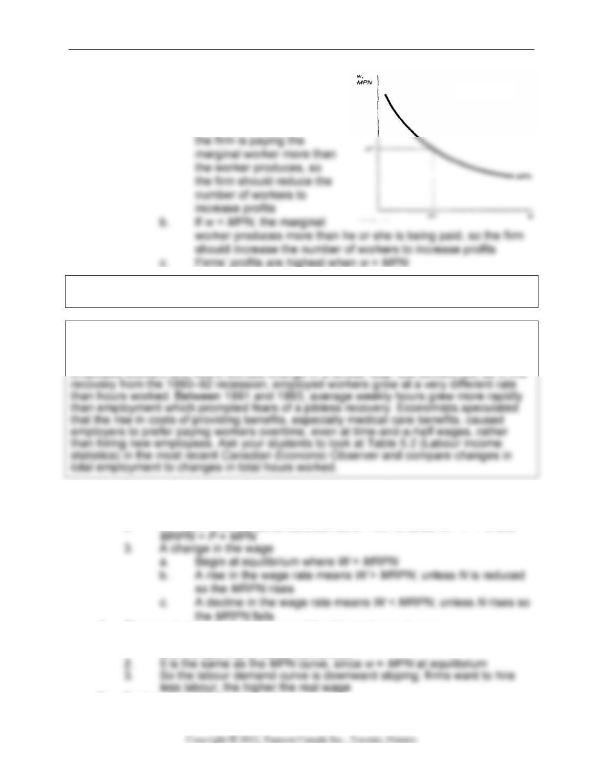
2. Analysis at the margin: costs and

benefits of hiring one extra worker

(Fig. 3.4; like text Fig. 3.5)

a. If real wage (w) > marginal

product of labour (MPN),

Numerical Problem 3 sets up an example in which students calculate MPN and see

what happens when the wage rate or price of the product change.

Data Application

We generally assume that when we speak of labour or employment we could be

referring to either the number of people employed or total hours worked. Generally, both

B. The marginal product of labour and labour demand

1. Example: The Clip Joint—setting the nominal wage equal to the

marginal revenue product of labour (MRPN = P x MPN)

2. W = MRPN is the same condition as w = MPN, since W = P × w and

C. The marginal product of labour and the labour demand curve

1. Labour demand curve shows relationship between the real wage rate

and the quantity of labour demanded

D. Factors that shift the labour demand curve

Figure 3.4

32 Chapter 3

E. Aggregate labour demand (Fig. 3.5)

1. Aggregate labour demand is

demand

III. The Supply of Labour (Sec. 3.3)

A. Supply of labour is determined by

individuals

1. Aggregate supply of labour is

sum of individuals’ labour

supply

3. Real wages and labour supply

a. A pure substitution

effect: A one day rise in

the real wage.

B. The labour supply curve (Fig. 3.6; like text Fig. 3.7)

1. Increase in the current real wage should raise quantity of labour

supplied

2. Labour supply curve relates quantity of labour supplied to real wage

Theoretical Application

The field of labour economics studies the determinants of labour supply. One of the

Productivity, Output, and Employment 33

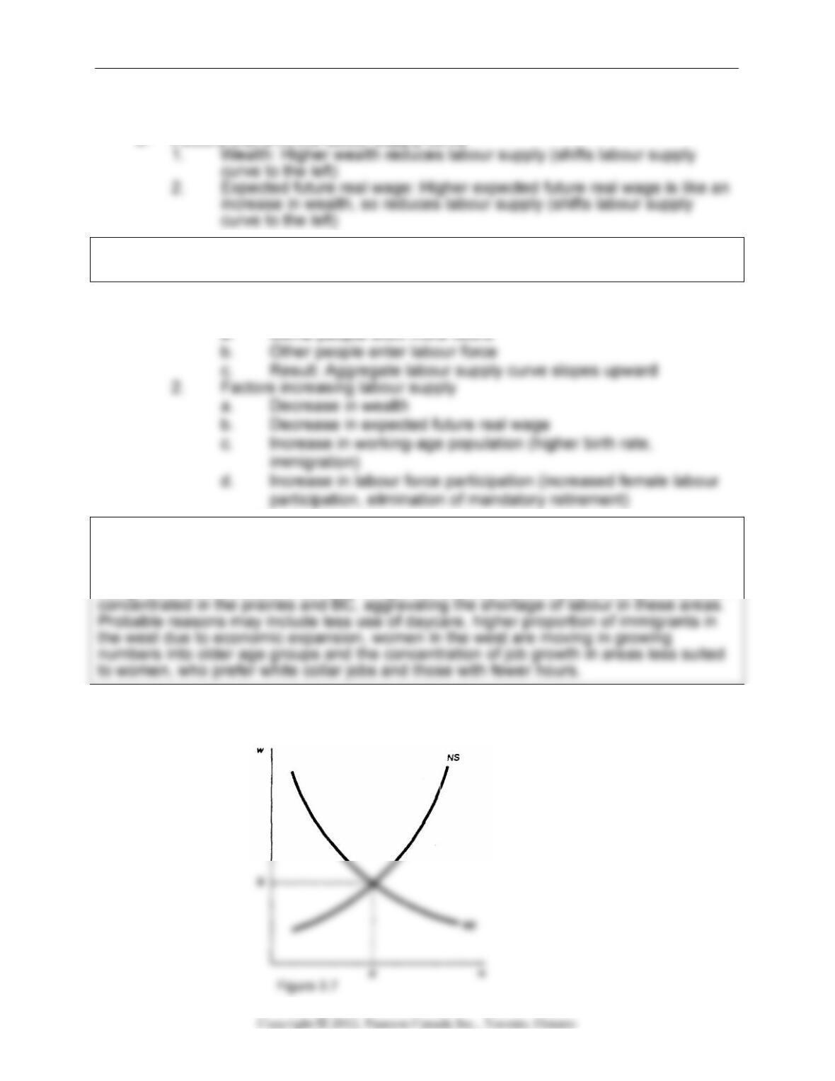
3. Labour supply curve slopes upward because a higher wage

encourages people to work more

C. Factors that shift the labour supply curve

Analytical Problem 4 asks students to think about factors that shift an individual’s labour

supply curve.

D. Aggregate labour supply

1. Aggregate labour supply rises when current real wage rises

Data Application

A broad characterization of labour force participation rates (LFPR) is that men’s LFPR

has declined fairly steadily over the past 60 years, while the LFPR of women has been

rising. But since 1990s, women’s LFPR growth slowed. Most of this slowdown has been

IV. Labour Market Equilibrium (Sec. 3.4)

A. Equilibrium: Labour supply equals labour demand (Fig. 3.7; Key Diagram 2;

like text Fig. 3.11)

34 Chapter 3

1. Classical model of the labour market—real wage adjusts quickly

2. Determines full-employment level of employment and market-

Data Application

What is full-employment output? For many of our theories about macroeconomics, we

need a measure of full-employment output, but it is not obvious where to get such a

measure. In practice, economists make some assumptions about the structure of the

economy, including the production function, apply these assumptions to the data, and

thus estimate what they think is the full-employment level of output.

C. Application: Output, employment, and the real wage during oil price shocks

1. Sharp oil price increases in 1973–74, 1979–80, 1990, 2008

2. Adverse supply shock—lowers labour demand, employment, the real

wage, and the full–employment level of output

D. Application: Technical change and wage inequality

1. Two important features of Canadian real wages since 1970

a. real wage growth has slowed

Data Application

There are, of course, many different wages in the economy; our model with just one

wage is a simplification. When economists look at real data to see how wages are

Numerical Problems 4, 5, and 6 are exercises in which students are given algebraic

labour demand and supply curves and are asked to find the equilibrium. Analytical

Problems 3 (dealing with wage rigidity) and 5 (dealing with tax on labour demand) are

comparative static exercises dealing with labour market equilibrium.

Productivity, Output, and Employment 35

V. Unemployment (Sec. 3.5)

A. Measuring unemployment

1. Categories: employed, unemployed, not in the labour force

2. Labour Force = Employed + Unemployed

B. Changes in employment status

1. Flows between categories

Numerical Problem 7 is a quantitative exercise using the unemployment and

employment concepts.

Data Application

C. How long are people unemployed?

1. Most unemployment spells are of short duration

a. Unemployment spell = period of time an individual is

2. Most unemployed people on a given date are experiencing

unemployment spells of long duration

3. Reconciling 1 and 2—numerical example:

a. Labour force = 100; on the first day of every month, two workers

become unemployed for one month each; on the first day of

people on a given date have long spells

D. Why there are always unemployed people

1. Frictional unemployment

a. Search activity of firms and workers due to heterogeneity

b. Matching process takes time

36 Chapter 3

c. Another cause: Reallocation of workers out of shrinking

industries or depressed regions; matching takes a long time

3. The natural rate of unemployment

a. ū = natural rate of unemployment; when output and employment

E. Relating output and unemployment : Okun’s Law(Sec. 3.6)

1. Okun’s Law: the percentage gap between potential and actual output

Productivity, Output, and Employment 37

ADDITIONAL ISSUES FOR CLASSROOM DISCUSSION

1. What Causes Productivity to Rise or Fall?

The production function treats total factor productivity as a “black box.” What are some

real-world factors that may cause one individual, firm, or country to be more

economically productive than another, given the same capital and labour inputs? Asking

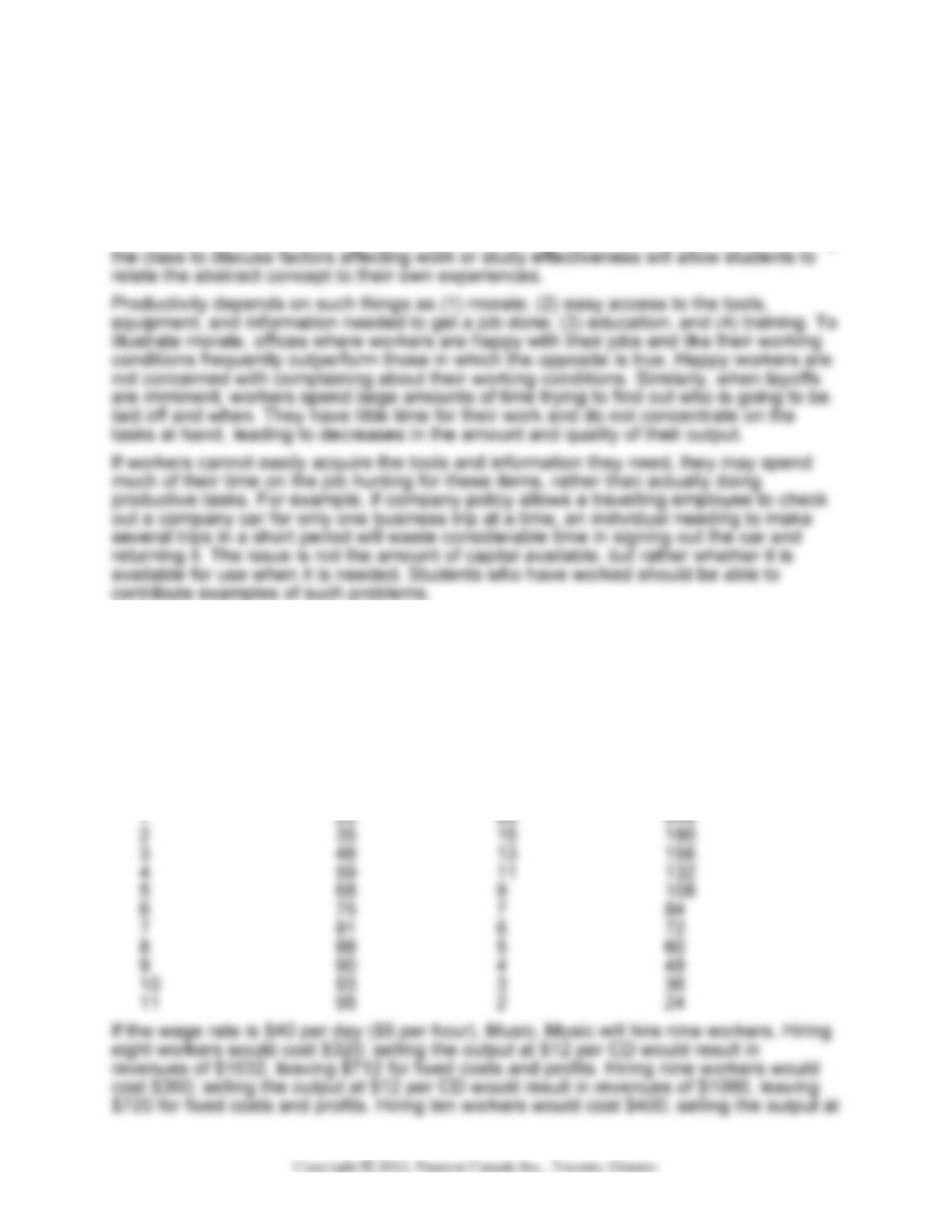
2. Another Production Function Example

Below is an example that is generally similar to Numerical Problem 3 at the end of the

chapter.

Music, Music

Number of Workers Compact Disks Marginal Product Marginal Revenue

Per Day Per Day of Labour Product

(units per day) (CD price $12)

0 0 — —

38 Chapter 3

3. How Do Society’s Expectations Affect Labour Supply?

The labour force participation rate varies substantially over time and across countries.

Other than the level of real wages, what factors contribute to this variation?

Besides real wages, a major determinant of labour supply is the needs and expectations

of the individuals in a society. During World War II many women worked to aid the war

4. Additional Costs and Benefits of Unemployment

What costs does unemployment impose on individuals and society? Are there any

potential benefits?

Productivity, Output, and Employment 39

Unemployment does provide some long-term benefits to the economy and individuals

despite the short-run hardships. In order to look for a new job, individuals frequently

assess their interests, skills, and experience. If they feel that their skills need updating,

workers may go to school to retrain and increase their skills and their chances of finding

a job. For example, white collar business workers who get laid off may decide to return

5. Is Technological Change Good for Workers?

Workers are often adamantly opposed to technological change; they see it as a threat to

their jobs. But technological change can make work easier and the higher productivity

allows higher wages to be paid.

Workers frequently oppose the introduction of new ways of producing goods and

services. From the Luddites in the 1800s, who smashed machines, to the 1990s

workers who fear computers, job holders have seen technology as a threat to their jobs