
Chapter 3 Productivity, Output, and Employment 49
◼ Answers to Textbook Problems
Review Questions
1. A production function shows how much output can be produced with a given amount of capital and
labor. The production function can shift due to supply shocks, which affect overall productivity.
2. The upward slope of the production function means that any additional inputs of capital or labor
produce more output. The fact that the slope declines as we move from left to right illustrates the idea
3. The marginal product of capital (MPK) is the output produced per unit of additional capital. The
4. The marginal revenue product of labor represents the benefit to a firm of hiring an additional worker,
while the nominal wage is the cost. Comparing the benefit to the cost, the firm will hire additional
workers as long as the marginal revenue product of labor exceeds the nominal wage, since doing so
5. The MPN curve shows the marginal product of labor at each level of employment. It is related to the
production function because the marginal product of labor is equal to the slope of the production
6. A temporary increase in the real wage increases the amount of labor supplied because the substitution
effect is larger than the income effect. The substitution effect arises because a higher real wage raises
the benefit of additional work for a worker. The income effect is small because the increase in the real

50 Abel/Bernanke/Croushore • Macroeconomics, Ninth Edition
7. The aggregate labor supply curve relates labor supply and the real wage. The principal factors shifting
the aggregate labor supply curve are wealth, the expected future real wage, the country’s working-age
8. Full-employment output is the level of output that firms supply when wages and prices in the economy
have fully adjusted; in the classical model of the labor market, this occurs when the labor market is in
9. The classical model of the labor market assumes that any worker who wants to work at the
equilibrium real wage can find a job, so it is not very useful for studying unemployment.
10. The labor force consists of all employed and unemployed workers. The unemployment rate is the
11. An unemployment spell is a period of time that a person is continuously unemployed. Duration is
the length of time of an unemployment spell. Two seemingly contradictory facts are that most
unemployment spells have a short duration and that most people who are unemployed at a particular
time are experiencing spells with long durations. These can be reconciled by realizing that there may
12. Frictional unemployment arises as workers and firms search to find matches. A certain amount of
frictional unemployment is necessary, because it is not always possible to find the right match right
13. Structural unemployment occurs when people suffer long spells of unemployment or are chronically
unemployed (with many spells of unemployment). Structural unemployment arises when the number

Chapter 3 Productivity, Output, and Employment 51
14. The natural rate of unemployment is the rate of unemployment that prevails when output and
employment are at their full-employment levels. The natural rate of unemployment is equal to the
15. Okun’s Law is a rule of thumb that tells how much output falls when the unemployment rate rises. It
is written either in terms of the levels of output and unemployment, as in Eq. (3.5), (
Y
− Y)/
Y
= 2
52 Abel/Bernanke/Croushore • Macroeconomics, Ninth Edition
Numerical Problems
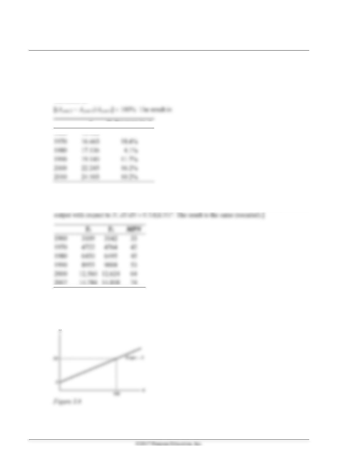
1. (a) To find the growth of total factor productivity, you must first calculate the value of A in the
production function. This is given by A = Y/(K.3N.7). The growth rate of A can then be
calculated as
A
% Increase in A
1960
1980
1990
2000
2010
(b) Calculate the marginal product of labor by seeing what happens to output when you add 1.0 to N;
call this Y2, and the original level of output Y1. [A more precise method is to take the derivative of
1960
1970
1980
1990
2000
2007
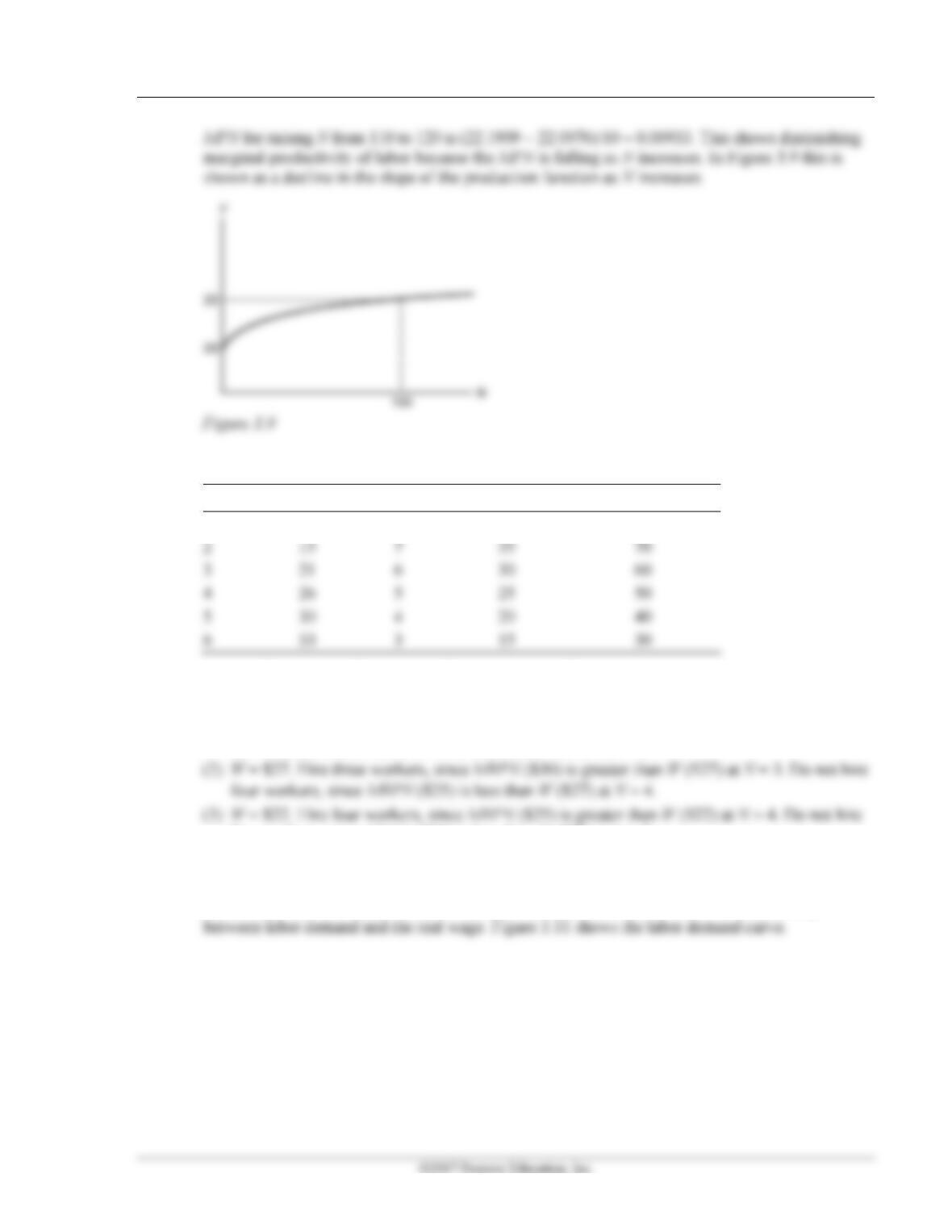
2. (a) The MPK is 0.2, because for each additional unit of capital, output increases by 0.2 units. The
slope of the production function line is 0.2. There is no diminishing marginal productivity of
capital in this case, because the MPK is the same regardless of the level of K. This can be seen
in Figure 3.8 because the production function is a straight line.
(b) When N is 100, output is Y = 0.2(100 + 100.5) = 22. When N is 110, Y is 22.0976. So the MPN for
raising N from 100 to 110 is (22.0976 − 22)/10 = 0.00976. When N is 120, Y is 22.1909. So the
Chapter 3 Productivity, Output, and Employment 53
3. (a)
N
Y
MPN
MRPN (P =
5)
MRPN (P =
10)
1
8
8
40
80
2
15
7
35
70
3
21
6
30
60
4
26
5
25
50
5
30
4
20
40
6
33
3
15
30
(b) P = $5.
(1) W = $38. Hire one worker, since MRPN ($40) is greater than W ($38) at N = 1. Do not hire
two workers, since MRPN ($35) is less than W ($38) at N = 2.
five workers, since MRPN ($20) is less than W ($22) at N = 5.
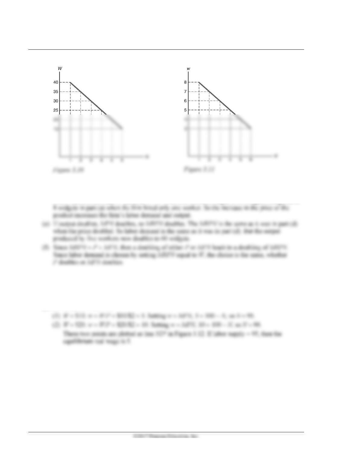
(c) Figure 3.10 plots the relationship between labor demand and the nominal wage. This graph is
different from a labor demand curve because a labor demand curve shows the relationship
54 Abel/Bernanke/Croushore • Macroeconomics, Ninth Edition
(d) P = $10. The table in part (a) shows the MRPN for each N. At W = $38, the firm should hire five
workers. MRPN ($40) is greater than W ($38) at N = 5. The firm shouldn’t hire six workers, since
MRPN ($30) is less than W ($38) at N = 6. With five workers, output is 30 widgets, compared to
4. MPN = A(100 − N)
(a) A = 1. MPN = 100 − N.
Chapter 3 Productivity, Output, and Employment 55
(b) A = 2. MPN = 2(100 − N).
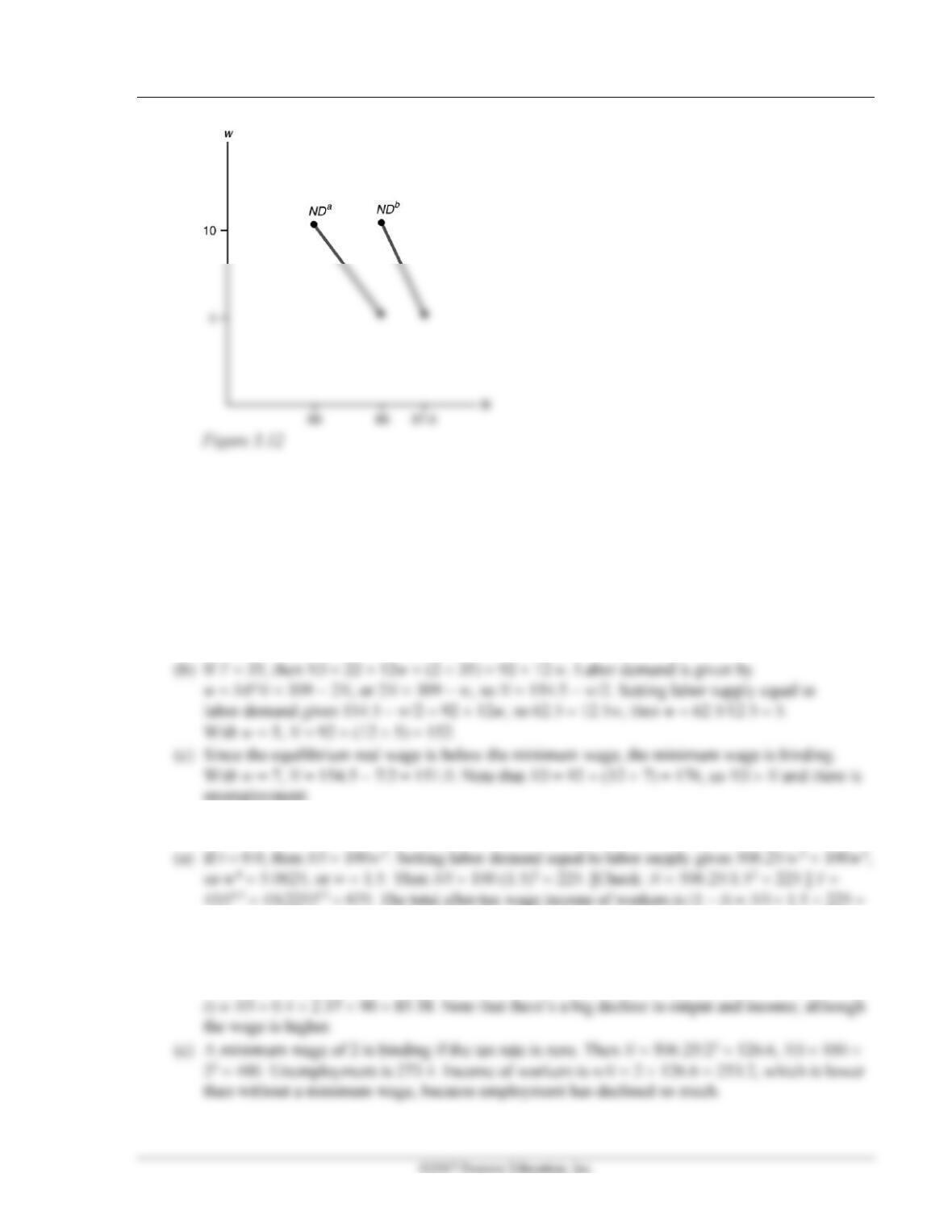
(1) W = $10. w = W/P = $10/$2 = 5. Setting w = MPN, 5 = 2(100 − N), so 2N = 195, so N = 97.5.
(2) W = $20. w = W/P = $20/$2 = 10. Setting w = MPN, 10 = 2(100 − N), so 2N = 190, so N = 95.
These two points are plotted as line NDb in Figure 3.12. If labor supply = 95, then the
equilibrium real wage is 10.
5. (a) If the lump-sum tax is increased, there’s an income effect on labor supply, not a substitution
effect (since the real wage isn’t changed). An increase in the lump-sum tax reduces a worker’s
wealth, so labor supply increases.
6. Since w = 4.5 K0.5 N−0.5, N−0.5 = 4.5 K0.5/w, so N = 20.25 K/w2. When K = 25, N = 506.25/w2.
337.5.
(b) If t = 0.6, then NS = 100 [(1 − 0.6) w]2 = 16w2. The marginal product of labor is MPN =
22.5/N0.5, so N = 100 [(1 − 0.6) 22.5/N0.5]2, so N2 = 8100, so N = 90. Then Y = 45N0.5 =
45(90)0.5 = 426.91. Then w = 22.5/900.5 = 2.37. The total after-tax wage income of workers is (1 −

56 Abel/Bernanke/Croushore • Macroeconomics, Ninth Edition
7. (a) At any date, 25 people are unemployed: 5 have lost their jobs at the start of the month and 20
have lost their jobs either on January 1 or July 1. The unemployment rate is 25/500 = 5%.
8. Number who become unemployed:
From not in the labor force: 2% of 93.0 million = 1.860 million
From employed: 1% of 148.8 million = 1.488 million
9. Since (
Y
− Y)
/Y
= 2(u −
u
), this can be rewritten as
Y
− Y = 2(u −
u
)
Y
or Y = [1 − 2(u −
u
)]
Y
, or
Y
= Y/[1 − 2(u −
u
)].
(a) Using the formula above, this table shows the value of
Y
, given values for u and Y.
Year
u
Y
Y
1
0.08
950
989.6
2
0.06
1030
1030.0
3
0.07
1033.5
1054.6
b. The first calculation of
Y/Y
comes from calculating the percent change in
Y
from part a.
The second calculation of Δ
Y/Y
comes from using Eq. (3.6): Y/Y =
Y/Y
− 2 u, so
Y/Y
=
Y/Y + 2 u.
Year
Y
Y/Y
YY
u
Y/Y
0.044
0.023

Chapter 3 Productivity, Output, and Employment 57
The two methods give fairly close answers.
10. (a) Total hours worked per week = 1900 workers 40 hours per worker = 76,000 hours per week.
Total output per week = 76,000 total hours per week 10 units of output per hour = 760,000
units of output. The unemployment rate is 100 unemployed/2000 labor supply = 0.05, or 5%.
0.0896) = 691,904. The Okun’s Law coefficient is the percent change in output divided by the
58 Abel/Bernanke/Croushore • Macroeconomics, Ninth Edition
Analytical Problems
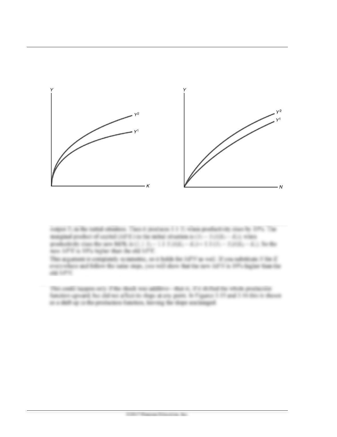
1. (a) See Figures 3.13 and 3.14.
Figure 3.13
Figure 3.14
(b) In the initial situation, capital K1 and labor N1 produce output Y1; when productivity rises they
produce output 1.1 Y1. Suppose that a small increase in capital to K2 with labor left at N1 produces
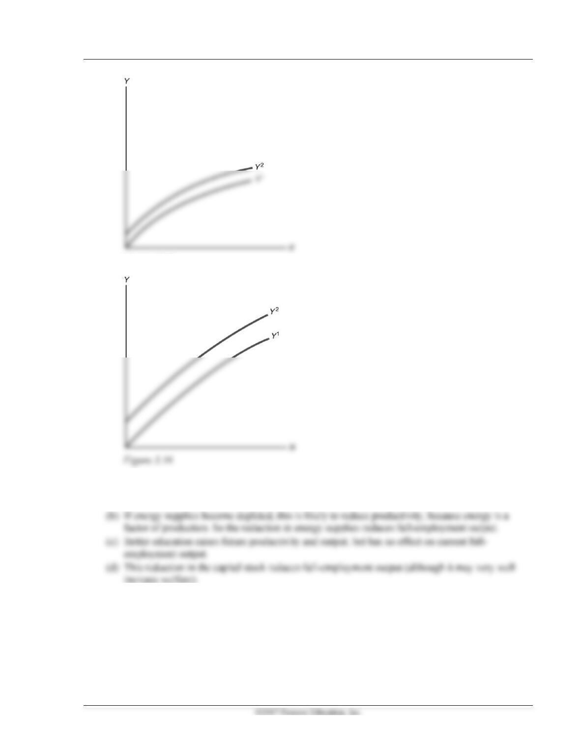
(c) Yes, it is possible for a beneficial productivity shock to leave the MPK and MPN unchanged.
Chapter 3 Productivity, Output, and Employment 59
Figure 3.15
2. (a) An increase in the number of immigrants increases the labor force, increasing employment and
increasing full-employment output.
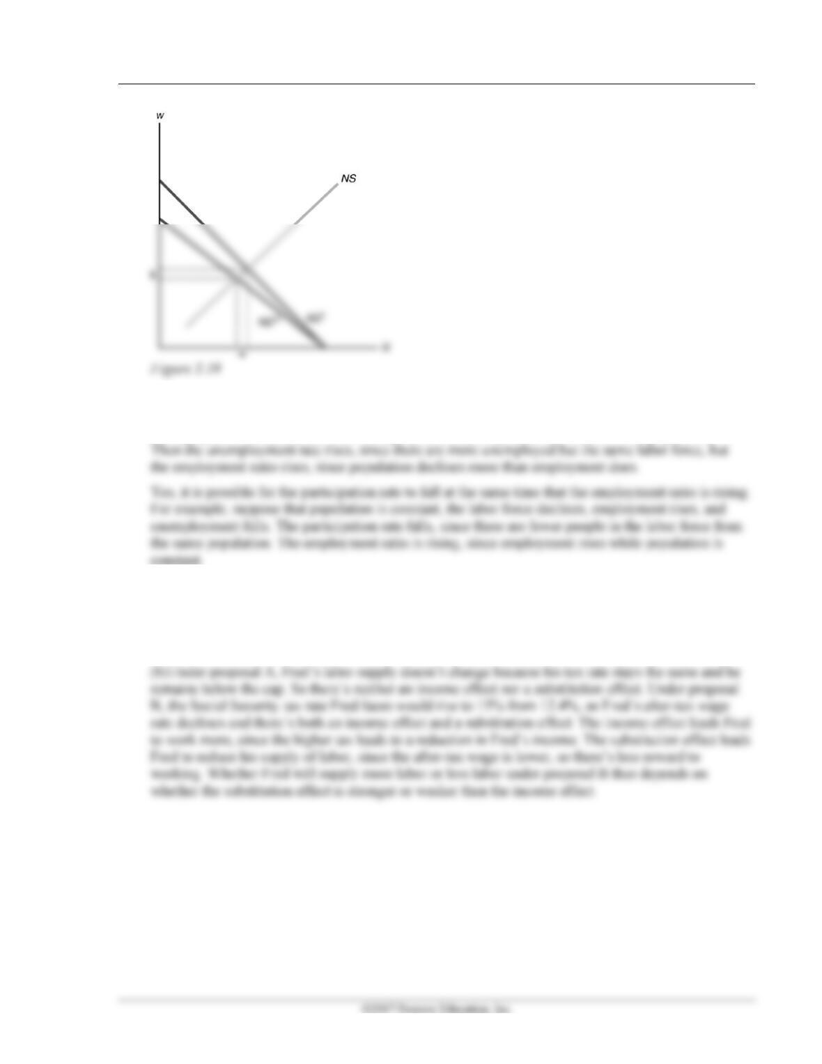
3. (a) As shown in Figure 3.17, when the real wage (w) is above its market-clearing level, labor supply
(NS) exceeds labor demand (ND). The difference is the amount of unemployment (U).

60 Abel/Bernanke/Croushore • Macroeconomics, Ninth Edition
4. (a) The increased value of Helena’s home increases her wealth. The rise in wealth leads to an income
effect that leads Helena to reduce her labor supply.
(b) The permanent rise in Helena’s real wage gives rise to offsetting income and substitution effects.
5. The tax reduces the marginal product of labor by 6%, since that portion of output goes to the
government rather than to the firm. Thus labor demand is reduced. With labor supply unchanged, the
Chapter 3 Productivity, Output, and Employment 61
6. Yes, it is possible for the unemployment rate and the employment ratio to rise during the same
month. For example, suppose the population falls, the labor force is constant, the number of
unemployed rises, and the number of employed falls (but by less than the decline in population).
7. (a) Since Sally earns $150,000 per year, she is above the cap, so the Social Security tax doesn’t affect
her after-tax wage (so there’s no substitution effect)—the higher tax only affects her income—and
thus has only an income effect. Since both proposals reduce Sally’s income by the same amount,
she’ll increase her labor supply by the same amount under both proposals.

62 Abel/Bernanke/Croushore • Macroeconomics, Ninth Edition
Working with Macroeconomic Data
1. Total factor productivity is generally rising over time. The growth rate of total factor productivity
2. Both the overall trend in the ratio of employment to the working-age population and the ratio of
the labor force to the working-age population generally increased from 1960 to 2000. Both the
3. Real full-employment GDP is smoother because it continues to grow during recessions, whereas