
Mishkin • Instructor’s Manual for The Economics of Money, Banking, and Financial Markets, Twelfth Edition 241
Chapter 22
ANSWERS TO QUESTIONS
1. Explain why the aggregate demand curve slopes downward and the short-run aggregate
supply curve slopes upward.
A rise in inflation causes monetary policymakers to raise the real interest rate. This reduces
2. Identify three factors that can shift the aggregate demand curve to the right and three different
factors that can shift the aggregate demand curve to the left.
3. “The appreciation of the dollar from 2012 to 2017 had a negative effect on aggregate demand
in the United States.” Is this statement true, false, or uncertain? Explain your answer.
The statement is correct. An appreciation of the U.S. dollar makes U.S. exports more
expensive for foreign consumers at the same time it makes imports into the U.S. cheaper. As
4. In many countries around the world, the population is aging and large segments of the
population are retiring or close to retirement. What effect would this have on a countries’
long-run aggregate supply curve? What will happen to income as a result?
5. If the labor force becomes more productive over time, how would the long-run aggregate
supply curve be affected?
6. Why are central banks so concerned with inflation expectations?
7. “If prices and wages are perfectly flexible, then Ȗ = 0 and changes in aggregate demand have
a smaller effect on output.” Is this statement true, false, or uncertain? Explain your answer.
8. What factors shift the short-run aggregate supply curve? Do any of these factors shift the
long-run aggregate supply curve? Why?
Shifts in the short-run aggregate supply curve result from changes in expected inflation, price
shocks, and persistent output gaps. None of these factors shift the long-run aggregate supply
9. If large budget deficits cause the public to think there will be higher inflation in the future,
what is likely to happen to the short-run aggregate supply curve when budget deficits rise?
10. In the aftermath of the financial crisis in the United States, labor mobility has decreased
significantly. How, if at all, might this affect the natural rate of unemployment?
11. When aggregate output is below the natural rate of output, what happens to the inflation rate
over time if the aggregate demand curve remains unchanged? Why?
When output is less than potential output, unemployment is above the natural rate and labor
market slack causes wages to rise less rapidly. As the Phillips curve suggests, this causes
12. Suppose the public believes that a newly announced anti-inflation program will work and so
lowers its expectations of future inflation. What will happen to aggregate output and the
inflation rate in the short run?
13. If the unemployment rate is above the natural rate of unemployment, holding other factors
constant, what will happen to inflation and output?
14. What happens to inflation and output in the short run and the long run when taxes decrease?
A decrease in taxes will lead to a rightward shift of the aggregate demand curve. In the short
run, inflation and output will both rise. This leads to tightness in the labor market, which
15. What factors led to decreases in both the unemployment and inflation rates in the 1990s?
Several factors led to an increase in potential output, which helped reduce the unemployment
rate and inflation rate. These included increased efficiencies in the health care industry, an
16. If stagflation is bad (high inflation and high unemployment), does this necessarily mean low
inflation and low unemployment is good?
Not necessarily. Even though low unemployment is desirable, if unemployment is too low
relative to the natural rate of unemployment, future inflation risk could build even if the
17. Why did the Federal Reserve pursue inherently recessionary policies in the early 1980s?
The Federal Reserve’s policies during that time were not intentionally recessionary; however,
they were necessary in order to reanchor inflation (and inflation expectations) at a permanently
18. In what ways is the Volcker disinflation considered a success? In what ways is it considered a
failure?
The Volcker disinflation is considered a success in that the Chair of the Federal Reserve, Paul
Volcker, was finally able to bring inflation down to a permanently lower, stable level after a
decade of high and volatile inflation through most of the 1970s. Unfortunately, the policies to
19.
Why
2007
–
Seve
r
fina
n
Unit
e
ANSW
E
20.
Usin
g
shor
t
a.
A
W
I
n
w
i
l
l
t
t
t
y
y
t
t
n
did China f
a
–
2009 finan
r
al factors p
l
n
cial crisis b
e
e
d States an
d
E
RS TO AP
P
g
an aggreg
a
t
run and th
e
A
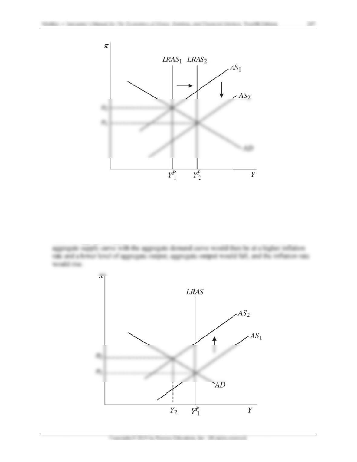
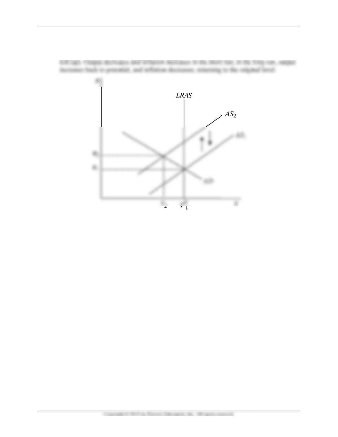
temporary
n
W
ith a temp
o
n
the short r
u
w
hich puts d
o
a
re much be
t
cial crisis?
l
ayed in fav
o
e
tter than th
e
d
the United
P
LIED PR
O
a
te demand
e
long run o
f
n
egative su
p
o
rary negati
v
u
n, output f
a
o
wnward pr
e
t
ter than th
e
o
r of China
t
e
United Sta
Kingdom i
n
O
BLEMS
and supply
g
f
the followi
n
p
ply shock.
v
e supply sh
o
a
lls and infl
a
e
ssure on th
e
e
United Sta
t
t
hat allowe
d
t
es or the U
n
n
general ar
e
g
raph, sho
w
n
g:
o
ck, the sho
r
a
tion rises.
T
e
inflation ra
t
t
es and the
U
d
them to we
n
ited Kingd
o
e
more close
w
and descri
b
r
t-run aggre
g
T
his creates
s
t
e. As labor
m
U
nited King
d
ather the ef
f
o
m. The ec
o
ly tied to th
e
b
e the effect
s
gate supply
s
lack in the
l
m
arket slac
k
d
om during
t
f
ects of the
o
nomies of t
h
e
functionin
g
s
in both the
curve shifts
l
abor marke
t
k
continues
a
t
he
h
e
g
of
e
up.
t
,
a
nd
Mishkin •
b.
A
W
t
h
l
a
s
u
a
n
21.
Supp
rese
a
p
rod
u
p
red
i
Tech
n
curv
e
I
nstructor’s Ma
n
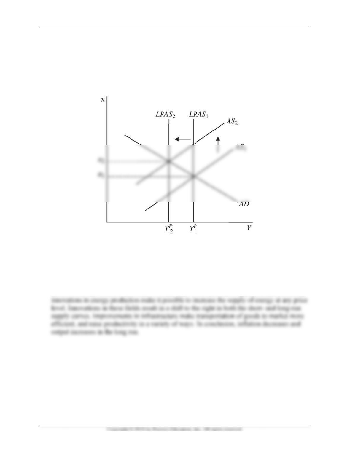
A
permanent
W
ith a perm
a
h
e left. This
a
bor market
u
pply curve
n
d inflation
o
se the Pre
s
a
rch and the
u
ctivity cha
n
i
ct the effect
s
n
ological c
h
e
. More fuel
–
n
ual for The Ec
o
negative su
p
a
nent negati
v
creates a co
n
tightens. A
s
shifts upwa
r
is higher at
t
s
ident gets
C
developme
n
n
ge for the
U
s
on inflatio
n
h
ange and in
f
–
efficient ca
r
o
nomics of Mon
e
p
ply shock.
v
e supply s
h
n
dition in w
h
inflation a
n
r
d to the ne
w
t
he new lon
g
C
ongress to
p
n
t of new tec
U
.S. econom
y
n
and outpu
t
f
rastructure
r
s result in
a
e
y, Banking, an
d
h
ock, the lon
g
h
ich output
n
d inflation
e
w
long-run e
g
-run equili
b
p
ass legislat
i
hnologies.
A
y
, use aggre
g
t
. Demonstr
a
improveme
n
a
decrease in
d
Financial Mar
k
g-run aggre
g
is now abo
v
e
xpectations
e
quilibrium.
b
rium.
i
on that enc
o
A
ssuming th
i
g
ate deman
d
a
te these ef
fe
n
ts affect th
e
the demand
k
ets, Twelfth E
d
g
ate supply
c
v
e potential
o
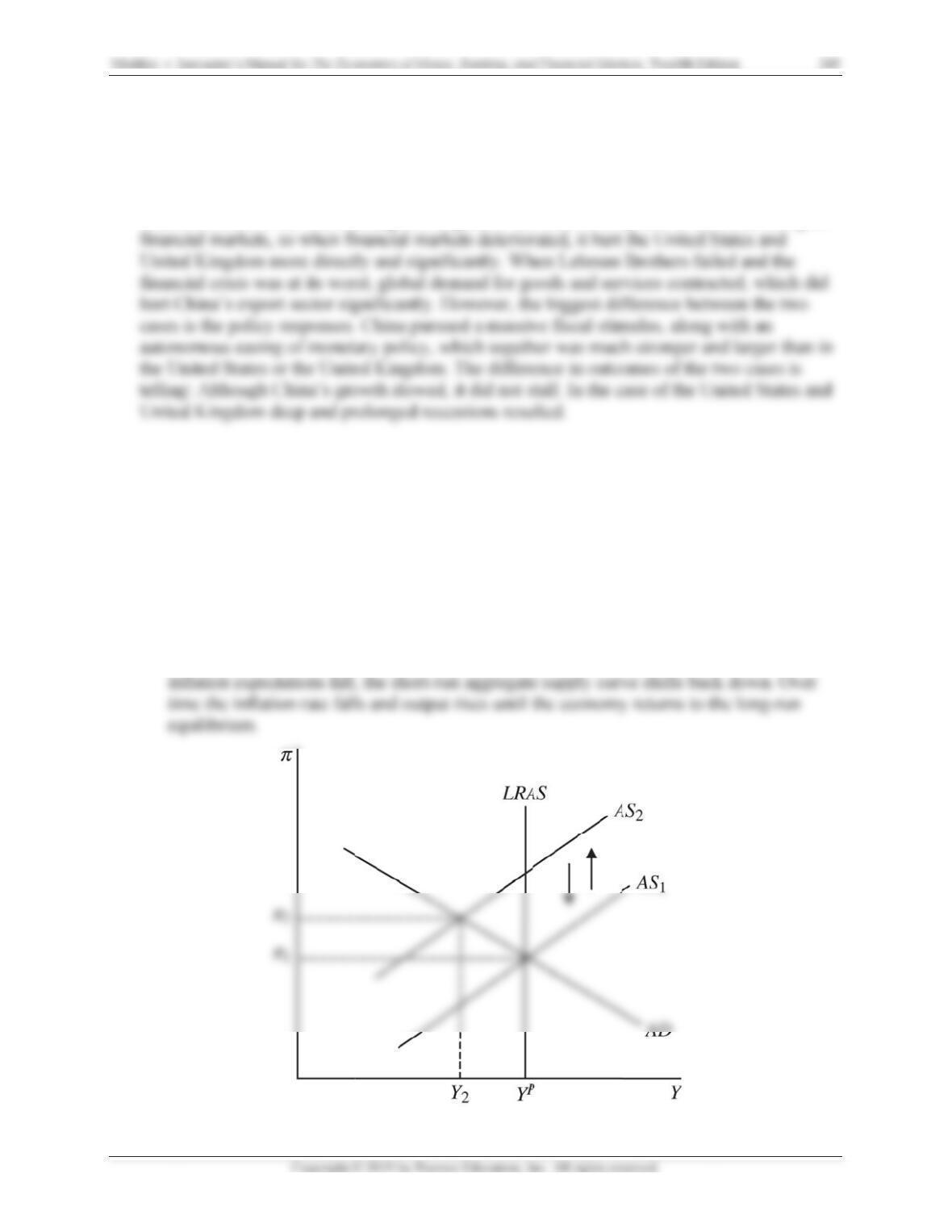
rise, the sh
o
Eventually,
o
urages inv
e
i
s policy lea
d
d
and suppl
y
fe
cts on a gr
a
e
long-run a
g
for gas at th
d
ition
c
urve shifts
o
utput, and
t
o
rt-run aggr
e
output is lo
w
e
stment in
d
s to a posi
t
y
analysis to
a
ph.
g
gregate su
p
e same time
246
to
t
he
e
gate
w
er
t
ive
p
ply
that
22.
Prop
Con
g
sho
w
dem
o
Beca
u
short
e
a
e
t
e
r
o
u
h
o
d
h
i
h
i
o
h
o
o
sals advoc
a
g
ress. Predi
c
w
ing the effe
c
o
nstrate thes
u
se goods
w
-run aggreg
a
a
ting the im
p
c
t the effects
c
ts on outpu
t
e effects.
w
ould cost
m
a
te supply c
u
p
lementatio
n
of such a t
a
t
and inflati
o
m
ore, the nati
u
rve would s
h
n
of a natio
n
a
x on the ag
g
o
n. Use a gr
a
onal sales t
a
h
ift to the le
n
al sales tax
gr
egate sup
p
a
ph of aggr
e
a
x would rai
ft. The inter
s
have been
p
p
ly and dem
a
e
gate suppl
y
se producti
o
s
ection of th
e
p
resented b
ef
a
nd curves,
y
and deman
o
n costs, an
d
e
short-run
ef
ore
d to
d
the
23.
Supp
une
m
scen
a
In or
d
aggr
e
24.
Clas
s
effec
t
a.
F
N
O
a
n
o
se the infl
a
m
ployment r
a
a
rio is possi
b
d
er for the
u
e
gate suppl
y
s
ify each of
t
t
s on inflati
o
F
inancial fri
c
N
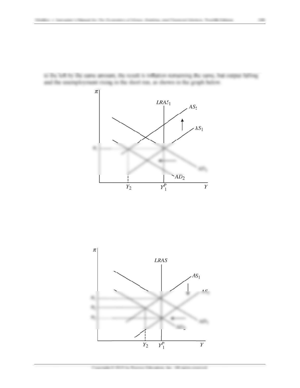
egative de
m
O
utput and i
n
n
d inflation
a
tion rate re
m
a
te increase
s
b
le.
u
nemployme
n
and deman
d
t
he followin
g
o
n and outp
u
c
tions incre
a
m
and shock.
n
flation fall
i
falls.
m
ains relati
v
s
. Using an
a
n
t rate to ris
d
curves wo
u
g
as a suppl
y
u
t in the sho
r
a
se.
An increase
i
n the short
r
v
ely consta
n
a
ggregate d
e
e and inflati
u
ld have to
s
y
shock or a
r
t run and i
n
in financia
l
r
un; in the l
o
n
t while out
p
e
mand and
s
i
on to remai
n
s
hift to the l
e
demand sh
o
n
the long ru
l
frictions re
d
o
ng run, out
p
p
ut decrease
s
s
upply grap
h
n
constant,
b
e
ft. If they s
h
o
ck. Use a g
r
u
n.
d
uces aggre
g
p
ut rises ba
c
s
and the
h
, show how
b
oth the
h
ift horizon
t
r
aph to sho
w
g
ate deman
d
c
k to potenti
a
this
t
ally
w
the
d
.
a
l,
Mishkin •
b.
H
P
i
n
o
u
c.
F
P
I
nstructor’s Ma
n
H
ouseholds
a
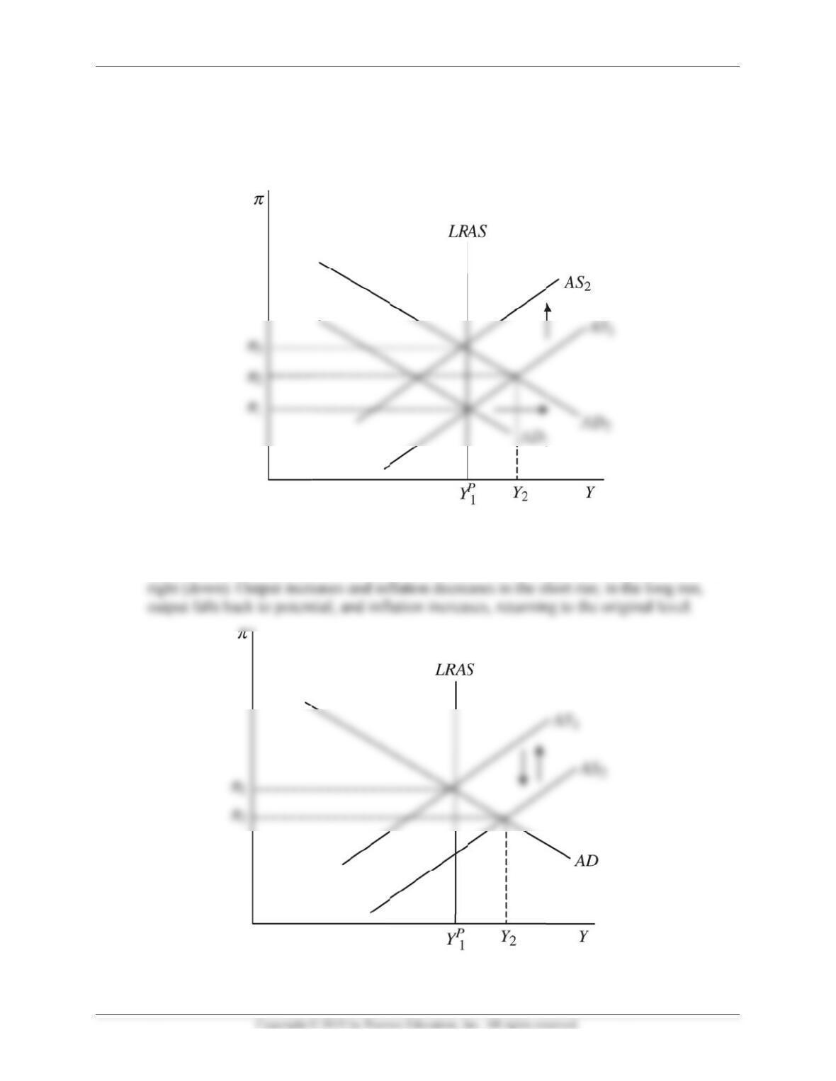
ositive dem
a
n
creases agg
r
u
tput falls b
a
F
avorable w
e
ositive (te
m
n
ual for The Ec
o
a
nd firms be
c
a
nd shock.
T
r
egate dema
n
a
c
k
to poten
t
e
ather prod
u
p
orary) sup
p
o
nomics of Mon
e
c
ome more
o
T
his increase
s
n
d. Output
a
t
ial, and inf
l
u
ces a recor
d
p
ly shock. T
e
y, Banking, an
d
o
ptimistic a
b
s
autonomo
u
a
nd inflation
l
ation increa
d
crop of w
h
his shifts th
e
d
Financial Mar
k
b
out the eco
n
u
s consumpt
i
increase in
t
ses.
h
eat and cor
n
e
short-run
a
k
ets, Twelfth E
d
n
omy.
i
on and inve
t
he short run
n in the Mi
d
a
ggregate s
u
d
ition
stment, whi
c
; in the long
d
west.
u
pply curve
t
249
c
h
run,
t
o the
u
a
t
l
l
g
g
Mishkin •
d.
A
N
I
nstructor’s Ma
n
A
uto worker
s
N
egative (te
m
n
ual for The Ec
o
s
go on strik
e
m
porary) sup
o
nomics of Mon
e
e
for four m
o
p
ly shock.
T
e
y, Banking, an
d
o
nths.
T
his shifts th
e
d
Financial Mar
k
e
short-run
a
k
ets, Twelfth E
d
a
ggregate su
p
d
ition
p
ply curve t
o
250
o
the
p
a
t
e
s
e
n
u
25.
Duri
n
way
o
infla
t
curv
e
If th
e
expe
c
the l
e
i
y
y
h
h
a
a
s
a
a
n
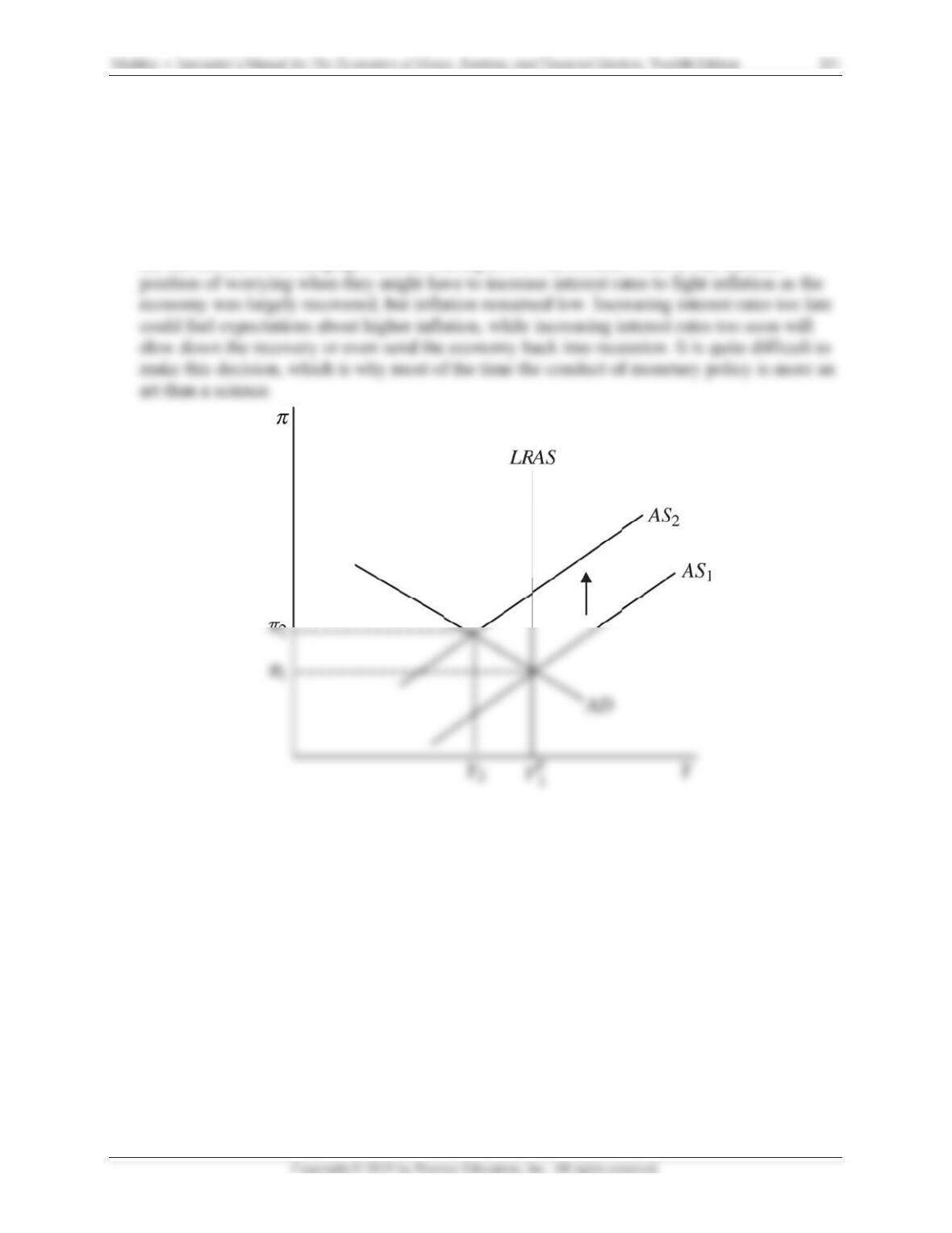
g 2017, so
m
o
f fighting
po
t
ion rates in
e
? Use an a
g
e
public ass
u
c
ted inflatio
n
e
ft (as show
n
m
e Fed offic
o
tential inc
r
the future,
w
g
gregate de
m
u
mes that th
e
n
will incre
a
n
in the gra
p
i
als discuss
e
r
eases in ex
p
w
hat would
b
m
and and s
up
e
current Fe
d
a
se, shifting
t
p
h below). D
e
d the possi
b
p
ected inflat
i
b
e the effect
up
ply graph
t
d
officials ar
t
he short-ru
n
uring 2017,
b
ility of incr
e
i
on. If the p
u
on the shor
t
t
o illustrate
y
e not that w
o
n
aggregate
Fed official
e
asing inter
e
u
blic came t
o
t
-run aggre
g
y
our answe
r
o
rried abou
t
supply curv
e
l
s were in th
e
e
st rates as
a
o
expect hig
h
g
ate supply
r
.
t
inflation,
e upward a
n
e
difficult
a
h
er
n
d to
Mishkin • Instructor’s Manual for The Economics of Money, Banking, and Financial Markets, Twelfth Edition 252
ANSWERS TO DATA ANALYSIS PROBLEMS
1. Go to the St. Louis Federal Reserve FRED database and find data on real government
spending (GCEC1), real GDP (GDPC1), taxes (W006RC-1Q027SBEA), and the personal
consumption expenditure price index (PCECTPI), a measure of the price level. Download all
of the data into a spreadsheet, and convert the tax data series into real taxes. To do this, for
each quarter, divide taxes by the price index and then multiply by 100.
a. Calculate the level change in real GDP over the four most recent quarters of data
available, and the four quarters prior to that.
See summary table below.
b. Calculate the level change in real government spending and real taxes over the four most
recent quarters of data available, and the four quarters prior to that.
See summary table below.
c. Are your results consistent with what you would expect? How do your answers to part (b)
help explain, if at all, your answer to part (a)? Explain using the IS and AD curves.
No, this is not consistent with what would be expected for tax and spending changes.
Over the most recent year period of 2016:Q1 to 2017:Q1, a contractionary fiscal policy
change took place with both government spending decreasing and taxes increasing. This
Gov’t Spending
Chg., $Bil.
Real Tax Chg.,
$Bil.
Real GDP Chg.,
$Bil.
2016:Q1 to 2017:Q1 6.6 28.02980553 331.6
2. Go to the St. Louis Federal Reserve FRED database and find data on the personal
consumption expenditure price index (PCECTPI), a measure of the price level; real
compensation per hour (COM-PRNFB); the nonfarm business sector real output per hour
(OPHNFB), a measure of worker productivity; the price of a barrel of oil (MCOILWTICO);
and the University of Michigan survey of inflation expectations (MICH). Use the frequency
setting to convert the oil price and inflation expectations data series to “Quarterly,” and use
the units setting to convert the price index to “Percent Change from Year Ago.” Download
all of the data into a spreadsheet, and convert the compensation and productivity measures
to a single indicator. To do this, for each quarter, take the compensation number and
subtract the productivity number. Call this difference “Net Wages Above Productivity.”
a. Calculate the change in the inflation rate over the four most recent quarters of data
available, and the four quarters prior to that.
See summary table below.
b. Calculate the changes in net wages above productivity, the price of oil, and inflation
expectations over the four most recent quarters of data available, and the four quarters
prior to that.
See summary table below.
c. Are your results consistent with what you would expect? How do your answers to part (b)
help explain, if at all, your answer to part (a)? Explain using the short-run aggregate
supply curve.
The data from part (b) move in somewhat different directions, so it is difficult to explain
the inflation behavior consistent with what would be expected to explain part (a). In the
most recent period, inflation expectations remained flat; oil prices increased (which
Inflation
Chg.
Inflation
Exp. Chg.
Oil Price
Chg., $/Brl. Net Wages Chg.
2016:Q1 to 2017:Q1 1.1 0.0 18.6 1.599