Basic Econometrics, Gujarati and Porter
227
CHAPTER 22:
TIME SERIES ECONOMETRICS: FORECASTING
22.1 As discussed in Sec. 22.1, broadly speaking there are five
22.2 Simultaneous-equation (SE) economic forecasting is based on a
system of equations (composed of at least two variables but usually
many more) that explain some economic phenomena on the basis of
22.4 Since the B-J method explicitly assumes that the underlying time
22.5 The B-J approach to forecasting is based on analyzing the
probabilistic properties of a single time series without relying on
22.6 It is a-theoretic because it uses less prior information than a SE
22.7 As we discussed in Exercise 22.1, there are five methods of
22.8 We want lags long enough to fully capture the dynamics of the
system being modeled. On the other hand, the longer the lags, the
228
22.9 See the answers to Exercises 22.2 and 22.6.
22.10 Operationally, the two procedures are similar. The difference comes
in the purpose of research. In Granger causality our objective is to
Empirical Exercises
22.11 The steps involved are as follows:
(1) Examine the series for stationarity. We have already seen that
(2) Examine the autocorrelation function (ACF) and the partial
(3) Having chosen an appropriate ARMA model, the next task is to
estimate it and examine the residuals of the estimated model. If
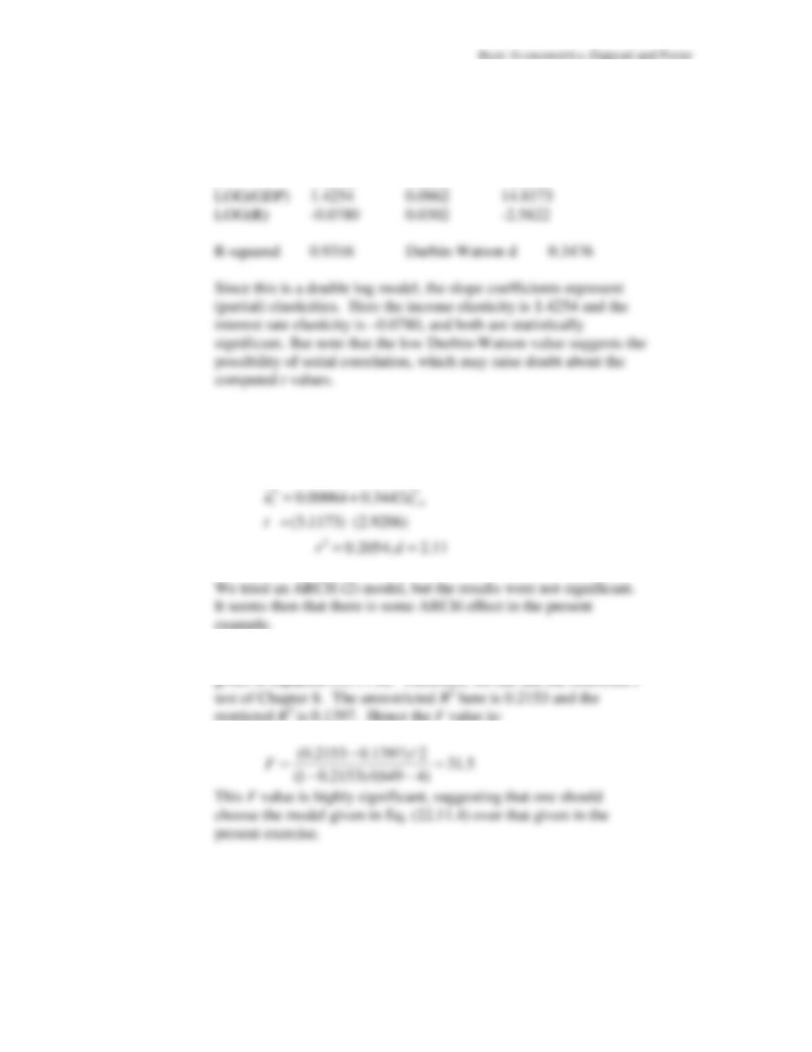
The regression results for the AR(4) model were as follows:
ln DPI
*
=0.0098 −0.1412 ln DPI
*
Basic Econometrics, Gujarati and Porter
229
22.12
Follow Exercise 22.11 and try the models MA(2), MA(6), AR(2)
22.13
Follow Exercise 22.11 and try the models MA(1) and AR(1), again
22.15
According to the Schwarz criterion, choose the model
that has the lowest value of Schwarz statistic. The same also
22.16
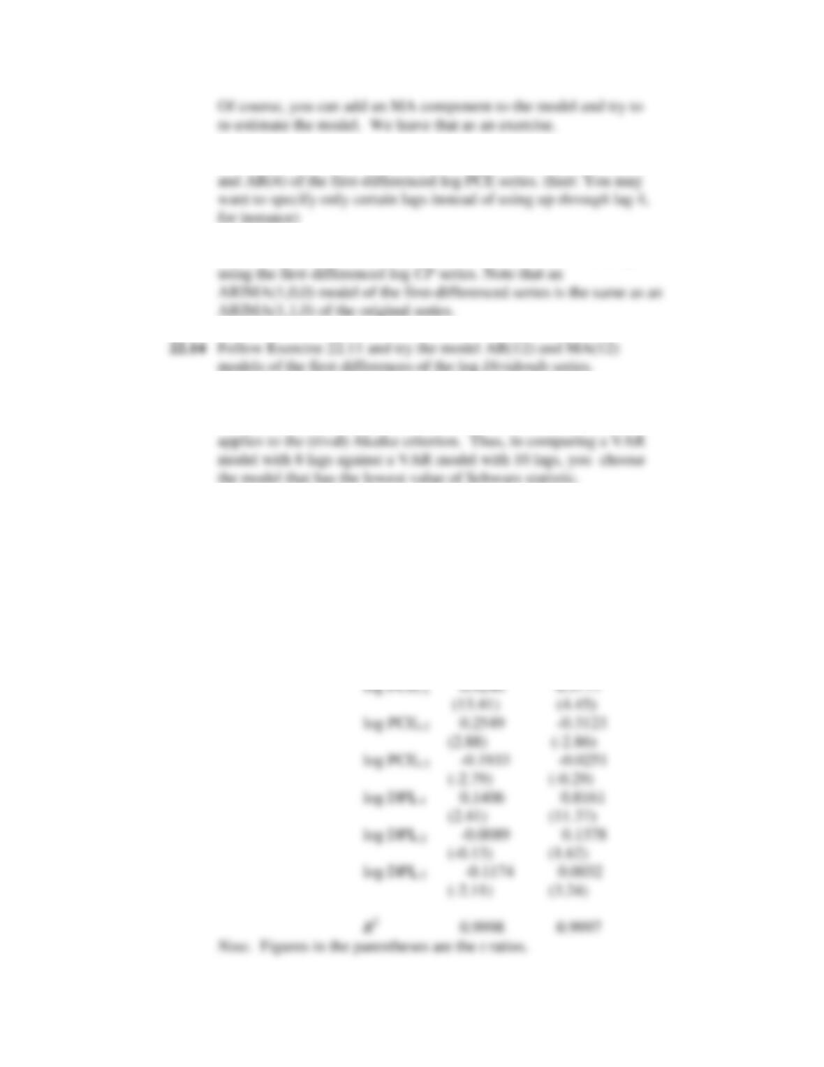
On the basis of the Schwarz criterion, it was determined that a
VAR model with 3 lags of log DPI and log PCE might suffice.
The regression results are as follows:
Dependent variable
→
log PCE log DPI
Explanatory Variables
↓
Intercept 0.0042 0.0319
(0.52
) (3.24)
Basic Econometrics, Gujarati and Porter
230
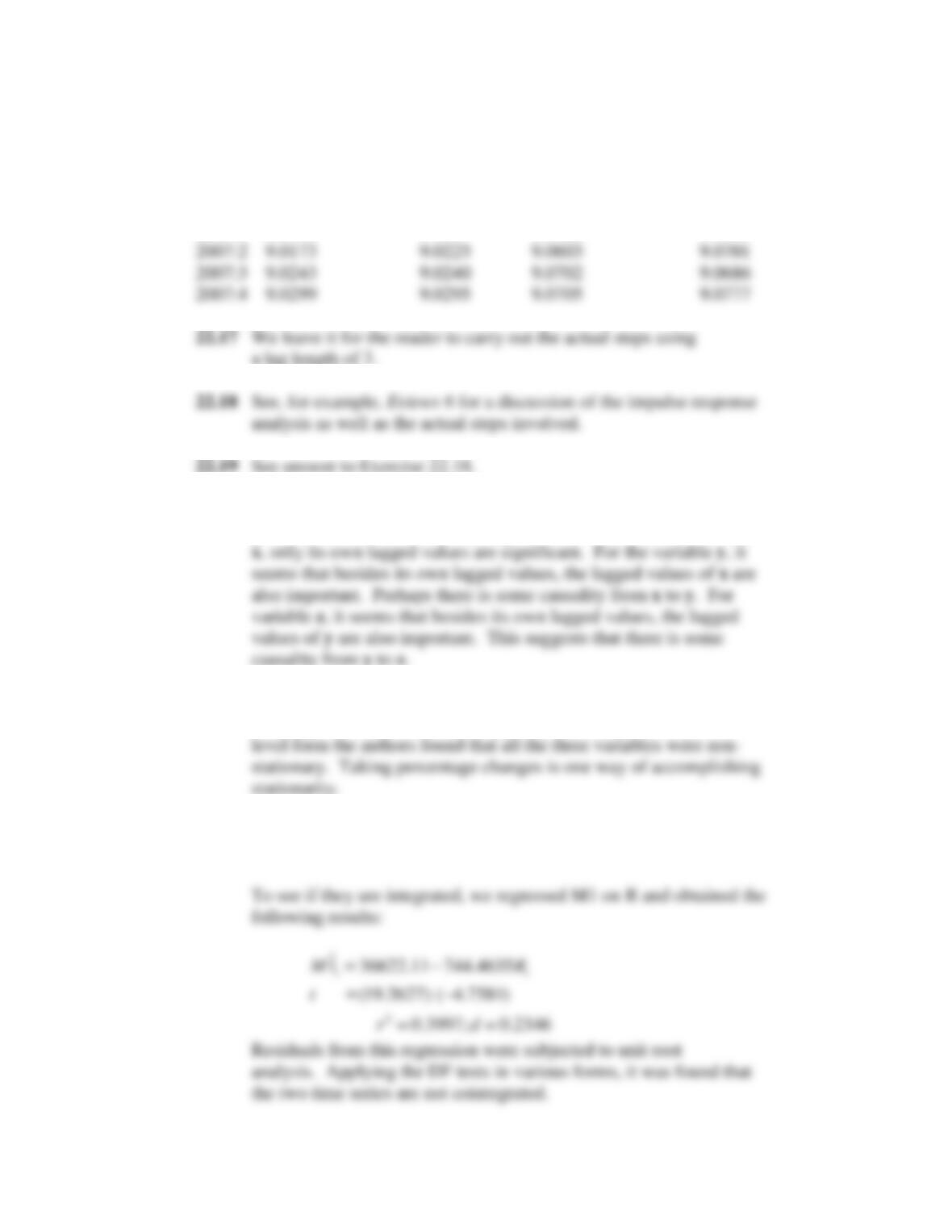
Based on this model, the actual and forecast values of the two
variables for 2007:1 to 2007:4 are as follows:
Q Actual log PCE Fcst log PCE Actual log DPI Fcst log DPI
2007:1 9.0138 9.0117 9.0623 9.0569
22.20
Although the model did not specifically test for causality, we can
get some idea about it from the reported F statistic. For the variable
22.21
For the application of the VAR methodology all the variables
entering into the model must be (jointly stationary). Perhaps in the
22.22
In the level form, M1 is nonstationary on the basis of the DF test
in its various forms. The same is true about R.
231
22.23
The regression results are as follows:
Variable Coefficient Std. Error t-Statistic
C -7.8618 1.2807 -6.1385
(b) To see if the ARCH effect is present, we obtained residuals (
ˆ
t
u
)
from the regression given in (a) and obtained the following
ARCH (1) regression:
22.24
The model given here is the restricted version of the model
232
22.25
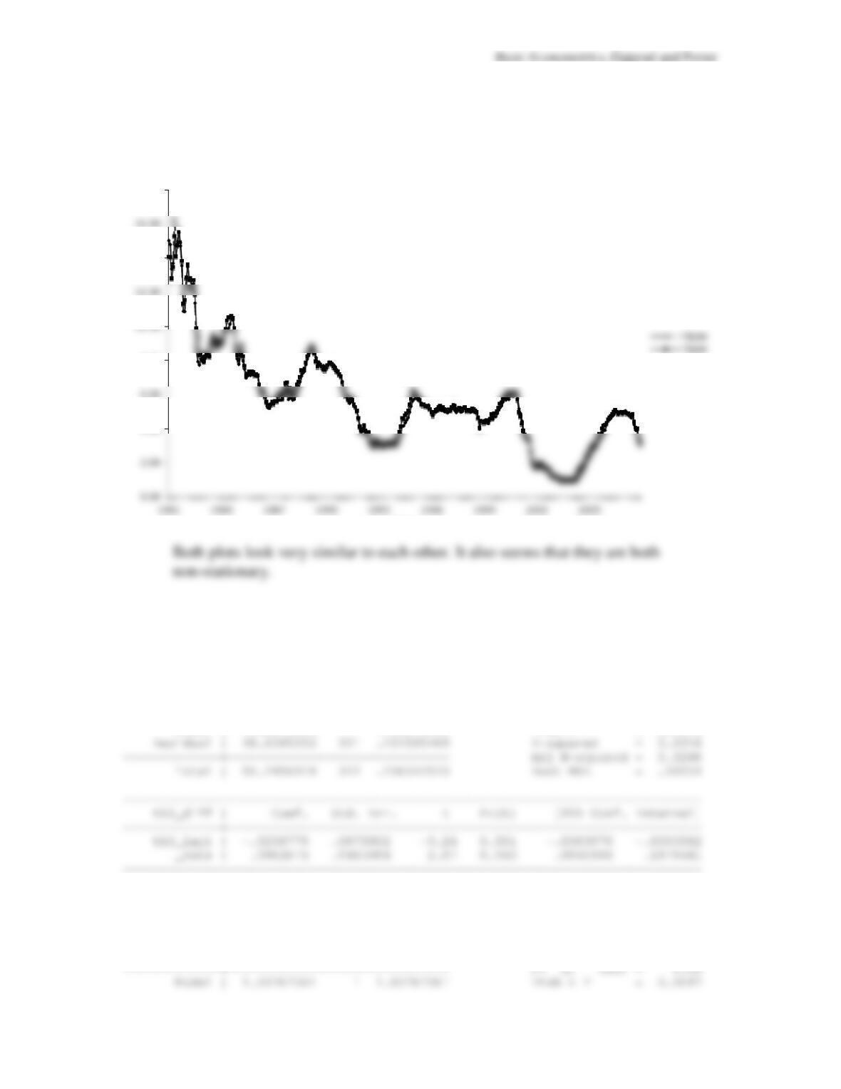
(a) Time series plot for the two series is:
(b) To perform the unit root test, we regressed the first differences
on the lagged series with the following results:
3-month Treasury Bills:
Source | SS df MS Number of obs = 323
————-+—————————— F( 1, 321) = 10.47
Model | 1.58675694 1 1.58675694 Prob > F = 0.0013
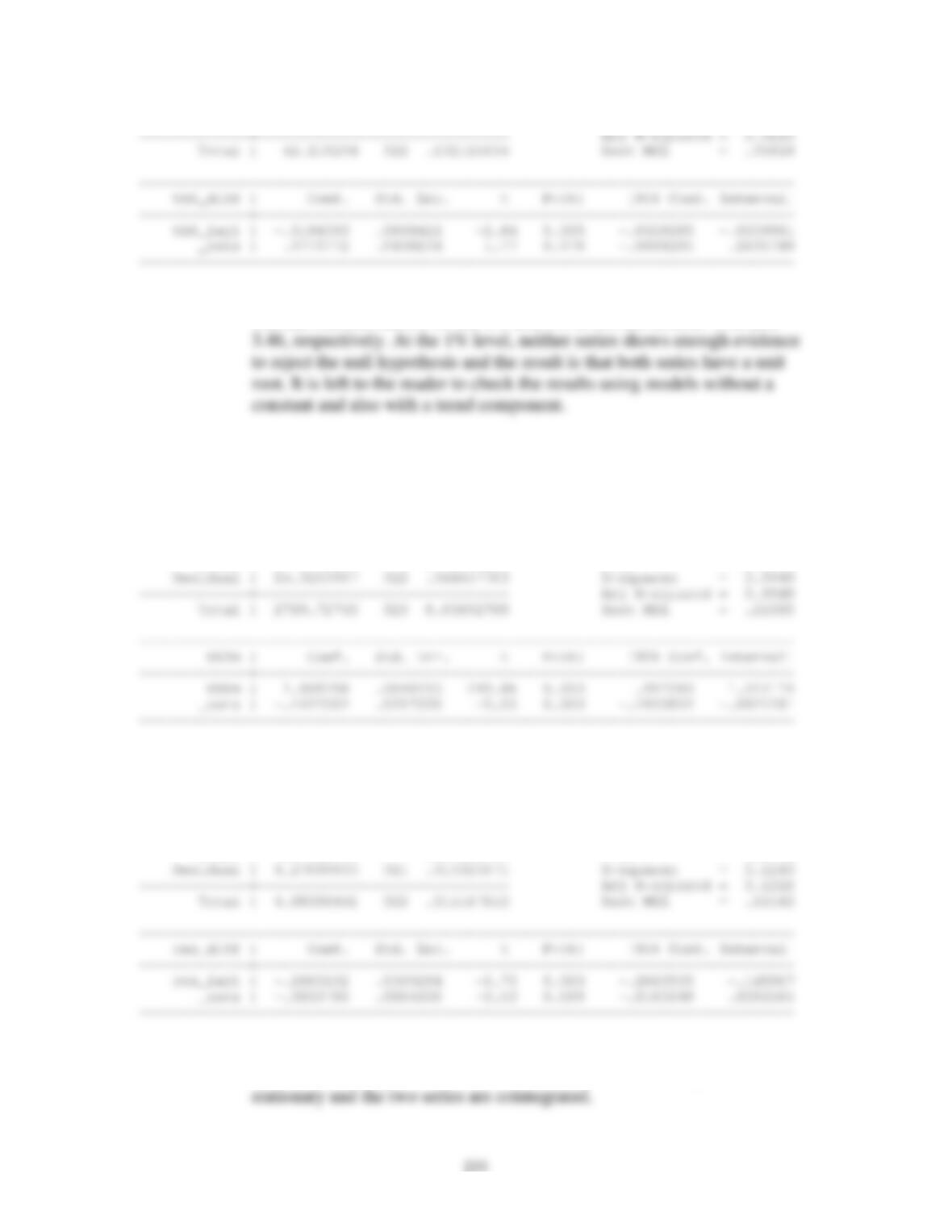
6-month Treasury Bills:
Source | SS df MS Number of obs = 323
3 and 6 Month Treasury Bills
4.00
8.00
14.00
18.00
Year
Basic Econometrics, Gujarati and Porter
Residual | 41.1815604 321 .128291465 R-squared = 0.0246
The tau statistic cutoffs for the 5% and 1% levels are around -2.88 and –
(c) To test if the two series are cointegrated, we will use the Engle-
Granger Test. First we estimate the residuals of the regression of 3-month
bills on 6-month bills:
Source | SS df MS Number of obs = 324
————-+—————————— F( 1, 322) =62428.06
Model | 2775.41205 1 2775.41205 Prob > F = 0.0000
and we saved the residuals from this regression. Now the regression of the
differenced residuals on the lagged residuals is as follows:
Source | SS df MS Number of obs = 323
————-+—————————— F( 1, 321) = 45.56
Model | .607086075 1 .607086075 Prob > F = 0.0000
The t statistic for the slope from this regression is -6.75, which is certainly
in the rejection region. Therefore, the residuals from this regression are

234
22.26
This is a class exercise.
22.27
This is a class exercise.