Chapter 22
The Firm: Cost and Output Determination
◼ Overview
The chapter begins by introducing the concepts of the short run and long run followed by a presentation
of the short-run production function. From the production function the law of diminishing returns is
developed. The law of diminishing returns is used to account for the general shape of most short-run cost
curves. Then the various cost concepts applied in later chapters are presented. The total, marginal, and
average cost curves are introduced. Next, the relationship between marginal and average curves is
presented. The chapter shows how to derive the firm’s long-run average cost curve and relates it to the
concepts of economies and diseconomies of scale.
◼ Learning Objectives
After studying this chapter, the student should be able to:
• 22.1 Discuss the difference between the short run and the long run from the perspective of a firm
◼ Outline
I. Short Run Versus Long Run: When dealing with suppliers (firms), there are two time periods for
analysis.
A. The Short Run: The short run is a time period when some inputs, such as plant size, cannot be
changed.
B. The Long Run: The long run is a time period in which all factors of production can be varied.
II. A Firm’s Production
A. The Relationship between Output and Inputs: The relationship between output and labor
and capital inputs is as follows: output per unit time period equals some function of capital and
labor inputs. Production is any activity that results in the conversion of resources into products.
It is a technological relationship.
1. The Production Function: A Numerical Example:
a. Properties of the Production Function: The production function specifies the
332 Miller • Economics Today, Nineteenth Edition
b. Total Product: Total output. (See Figure 22-1.)
2. Average and Marginal Physical Product: Average physical product is total product
B. Diminishing Marginal Product: The law of diminishing marginal product is the observation
that successive increases in a variable factor of production, such as labor, added to fixed factors
of production will reach a point beyond which the extra or marginal product that can be
attributed to each additional unit of the variable factor of production will decline.
(See Figure 23-1.)
1. Measuring Diminishing Marginal Product: The analysis is limited to one variable factor
of production. Every other factor of production is held constant. Marginal returns are
referred to as the marginal product (MP).
a. Initially Increasing Marginal Product: As output increases, at first it is possible for
2. An Example of the Law of Diminishing Marginal Product: An example of the law of
diminishing marginal product is presented in this section.
1. Graphing the Marginal Product of Labor: A set of hypothetical numbers is
III. Short-Run Costs to the Firm: In the short run, some inputs are fixed, and some are variable. Total
A. Total Fixed Costs: Costs that do not vary with output. (See Figure 22-2 for a worked out
example of costs and cost curves.)
B. Total Variable Costs: Costs that vary with the rate of production.
C. Short-Run Average Cost Curves
1. Average Fixed Costs (AFC): Total fixed costs divided by quantity produced.
2. Average Variable Costs (AVC): Total variable cost divided by quantity produced.
D. Marginal Cost: The change in total costs due to a change in production of one unit, i.e., the
E. The Relationship between Average and Marginal Costs: There is always a definite
relationship between average costs and marginal costs.
1. Average Variable Costs and Marginal Costs: When marginal cost is less than average
2. Average Total Costs and Marginal Costs: When marginal cost is less than average total
F. Minimum Cost Points: The marginal cost curve intersects the minimum point of the average
G. The Relationship between Diminishing Marginal Product and Cost Curves
(See Figure 22-3.)
1. Average Costs and Average Product
b. Evaluating the Shapes of the AVC and ATC Curves: AVC decreases as AP
H. Marginal Cost and Marginal Product
1. Computing Marginal Cost: MC = change in total cost/change in output. If labor is the
only variable input and the wage is constant, then MC = W/MP.
2. Explaining the Shape of the Marginal Cost Curve: Short-run firm cost curves reflect the
law of diminishing marginal product. Given a constant price of a variable input, MC
IV. Long-Run Cost Curves: The long run is a time period during which full adjustment can be made
to any change in the economic environment. (See Figure 22-4.)
A. The Firm’s Planning Horizon: In the long run, all factors of production are variable. Long-
B. Long-Run Average Cost Curve: This curve is the locus of points representing the minimum
unit cost of producing any given rate of output, given current technology and resource prices,
and also the planning curve.
C. Why the Long-Run Average Cost Curve Is U-Shaped: The reason it is U-shaped is
economies of scale that occur when output increases lead to decreases in long-run average
1. Reasons for Economies of Scale
a. Specialization: As a firm’s scale of operation increases, the opportunities for
specialization in the use of resource inputs also increase.
334 Miller • Economics Today, Nineteenth Edition
d. Why a Firm Might Experience Diseconomies of Scale: One of the basic reasons that
D. Minimum Efficient Scale: The lowest rate of output per unit time period at which average
◼ Points to Emphasize
The Law of Diminishing Marginal Product
Although the law of diminishing marginal product has implications for costs and profits, it is best
understood as a technological statement: It relates inputs to outputs. It is important to point out that the
The Law of Diminishing Marginal Product Is a Short-Run Concept
The law of diminishing returns can be applied to a firm only in the short run. The firm can increase output
in the short run only by adding more and more labor; other inputs are held constant by assumption. Thus,
the law predicts that eventually the marginal product of labor will fall.
The first key relationship occurs between a declining marginal product of labor and an increasing marginal
cost. One way to show this relationship is to construct a table with quantity of labor in hours in the first
Economies of Scale
Economies of scale refer to what happens to the long-run average cost curve. If plant size rises and average
Chapter 22 The Firm: Cost and Output Determination 335
Short Run versus the Long Run
An understanding of both production and cost requires an understanding of the short run and the long run. For
◼ For Those Who Wish to Stress Theory
Marginal and Average Cost
A key to understanding the shapes of the cost curves is the relationship between a marginal and an
average. The basic concept is simple. If a marginal value is below the average, the average is falling. If a
Sunk versus Variable Costs
It is crucial to be able to distinguish between sunk and variable (or marginal) costs. Economists maintain that
decisions should be made on future, not past, considerations. One who wishes to maximize must compare
marginal costs and marginal benefits. Fixed, or sunk, costs have already occurred and therefore are irrelevant
to present decision making. For example, ask your students if they own season tickets for a concert or athletic
series. If that season ticket has already been purchased, it is a sunk cost and would not influence a rational
◼ Further Questions for Class Discussion
1. Ask students to explain the effect of an increase in total fixed costs on the marginal cost curve.
2. Why would the existence of diminishing marginal product result in U-shaped average variable
and average total cost curves? Diminishing marginal product results in marginal costs that
3. Given the fact that businesses are operated on a day-to-day basis in the short run, of what use is
the concept of long-run average cost to an entrepreneur? It is important for students to understand
4. Crime and violence have been at the top of Americans’ concerns for more than a decade. One
popular law aimed at reducing crime is called “three strikes and you’re out.” A defendant
with a prior conviction for two serious or violent offenses faces a mandatory life sentence for
conviction of a third offense. Suppose a felon is in the act of committing an armed robbery and a
5. According to the pharmaceutical industry, the average cost of developing a new drug is about
$800 million. What is the marginal cost to a pharmaceutical firm of producing the first dose of a
6. Suppose that an ISP leases a new server in order to increase the speed of Internet service by
increasing the bandwidth that is available to its customers. Would the cost of this lease increase
Chapter 22 The Firm: Cost and Output Determination 337
◼ Answers to Questions for Critical Analysis
Is a Firm’s Feasible Output Greater with Individual– or group-Structured Tasks?
(p. 488)
There is an old saying that “two heads are better than one.” Why might this saying be more likely
to hold true in producing output when the two heads involved are acquainted and have experience
with tasks than when they seek to produce output after randomly getting together?
Reducing Variable Costs by Initially Keeping the Bubbles Out of Bubble Wrap®
(p. 492)
Are the annual expenses that a shipper must incur to maintain its iBubble Wrap® air pumps part of
its fixed costs or of its variable costs?
Short-Run Average and Marginal Costs Increase at the World’s Ports (p. 495)
As ports have produced higher quantities of loading and unloading services, have there been
upward movements along their AVC and MC curves or upward shifts in those curves? Explain
A Government Produces Solar Energy on a Massive Scale—To Pump More Oil
(p. 502)
What would likely happen to long-run average cost at Oman’s facility if engineers encountered
difficulties in maintaining the facility’s substantial daily volume of oil production? Explain.
Tesla’s Initial Home-Battery Production Scale Is Below the Minimum Efficient
Scale (pp. 503–504)
If Tesla were to produce only a few dozen home batteries per month, would the company
experience economies of scale or diseconomies of scale? Explain.
338 Miller • Economics Today, Nineteenth Edition
◼ You Are There
Wal-Mart Relearns How to Reduce “Shrink” Costs (p. 504)
1. In your view, is a retailing firm’s shrink likely to contribute mostly to its fixed costs or
variable costs? Explain your reasoning.
2. Given that hiring and paying asset-protection customer specialists at all stores will push up
Walmart’s labor costs, what is McMillon assuming about the cost savings that can be
yielded by reducing Walmart’s shrink?
◼ Issues and Applications
Cutting Per-Unit Costs of Making Drugs and Exploring Other Worlds with 3D and
Molecular Printers (pp. 504–505)
1. If short-run average variable costs and marginal costs decline at every feasible quantity
of output, what (if anything) happens to the positions of the AVC, AFC, ATC, and
MC curves? Explain.
2. If long-run average costs decrease at each possible quantity, does the minimum efficient
scale necessarily either increase or decrease? Explain your reasoning?
◼ Research Project
1. For more information about the use of molecular printing in the design of chemical compounds for
◼ Answers to Problems
22-1. The academic calendar for a university is August 15 through May 15. A professor commits
to a contract that binds her to a teaching position at this university for this period. Based on
this information, explain the short run and long run that the professor faces.
Chapter 22 The Firm: Cost and Output Determination 339
22-2. The short-run production function for a manufacturer of flash memory drives is shown in
the table below. Based on this information, answer the following questions.
Input of Labor
(workers per week)
Total Output of
Flash Memory Drives
0
0
1
25
2
60
3
85
4
105
5
115
6
120
a. Calculate the average product at each quantity of labor.
b. Calculate the marginal product of labor at each quantity of labor.
c. At what point does marginal product begin to diminish?
Input of Labor
(workers per month)
Total Output of Flash
Memory Drives
Average Product
(a)
Marginal Product
(b)
0
0
—
—
1
25
25.00
25
2
60
30.00
35
3
85
28.33
25
4
105
26.25
20
5
115
23.00
10
22-3. During the past year, a firm produced 10,000 laptop computers. Its total costs were
$5 million, and its fixed costs were $2 million. What are the average variable costs of this
firm?
22-4. During the previous month, a firm produced 250 tablet devices at an average variable cost
of $40 and at an average fixed cost of $10. What were the firm’s total costs during the
month?
22-5. Just before the firm discussed in Problem 22-4 produced its last tablet device in the
previous month, its total costs were $12,425. What was the marginal cost incurred by the
firm in producing the final tablet device that month?
22-6. The cost structure of a manufacturer of microchips is described in the table at the next
column. The firm’s fixed costs equal $10 per day. Calculate the average variable cost,
average fixed cost, and average total cost at each output level.
Output
(microchips
per day)
Total Cost of
Output
($ thousands)
0
10
25
60
50
95
75
150
100
220
125
325
150
465
Output
(microchips
per month)
Total Cost of
Output
($ thousands)
Average
Total Costs
($ per unit)
Average
Fixed Costs
($ per unit)
Average
Variable Costs
($ per unit)
0
10
—
—
—
60
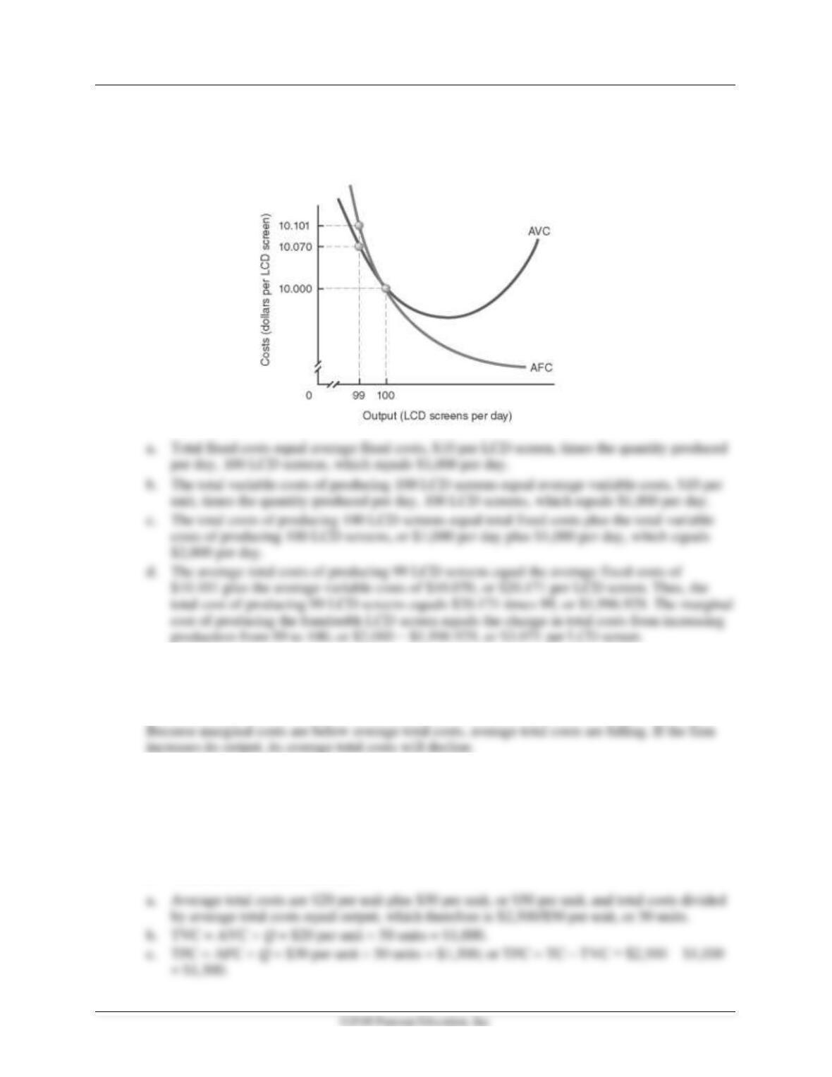
22-7. The diagram below displays short-run cost curves for a facility that produces liquid crystal
display (LCD) screens for cell phones:
a. What are the daily total fixed costs of producing LCD screens?
b. What are the total variable costs of producing 100 LCD screens per day?
c. What are the total costs of producing 100 LCD screens per day?
Chapter 22 The Firm: Cost and Output Determination 341
d. What is the marginal cost of producing 100 LCD screens instead of 99? (Hint: To
answer this question, you must first determine the total costs—or, alternatively, the
total variable costs—of producing 99 LCD screens.)
22-8. A watch manufacturer finds that at 1,000 units of output, its marginal costs are below
average total costs. If it produces an additional watch, will its average total costs rise, fall, or
stay the same?
22-9. At its current short-run level of production, a firm’s average variable costs equal $20 per
unit, and its average fixed costs equal $30 per unit. Its total costs at this production level
equal $2,500.
a. What is the firm’s current output level?
b. What are its total variable costs at this output level?
c. What are its total fixed costs?
22-10. In an effort to reduce their total costs, many companies are now replacing paychecks with
payroll cards, which are stored-value cards onto which the companies can download
employees’ wages and salaries electronically. If the only factor of production that a
company varies in the short run is the number of hours worked by people already on its
payroll, would shifting from paychecks to payroll cards reduce the firm’s total fixed costs
or its total variable costs? Explain your answer.
22-11. During autumn months, passenger railroads across the globe deal with a condition called
slippery rail. It results from a combination of water, leaf oil, and pressure from the train’s
weight, which creates a slippery black ooze that prevents trains from gaining traction.
a. One solution for slippery rail is to cut back trees from all of a rail firm’s rail network on
a regular basis, thereby helping to prevent the problem from developing. If incurred,
would this railroad expense be a better example of a fixed cost or a variable cost? Why?
b. Another way of addressing slippery rail is to wait until it begins to develop. Then the
company purchases sand and dumps it on the slippery tracks so that trains already en
route within the rail network can proceed. If incurred, would this railroad expense be a
better example of a fixed cost or a variable cost? Why?
22-12. In the short run, a firm’s total costs of producing 100 units of output equal $10,000. If it
produces one more unit, its total costs will increase to $10,150.
a. What is the marginal cost of producing 101 instead of 100 units of output?
b. What is the firm’s average total cost of producing 100 units?
c. What is the firm’s average total cost of producing 101 units?
22-13. Suppose that a firm’s only variable input is labor, and the constant hourly wage rate is $20
per hour. The last unit of labor hired enabled the firm to increase its hourly production
from 250 units to 251 units. What was the marginal cost of producing 251 units of output
instead of 250?
22-14. Suppose that a firm’s only variable input is labor. The firm increases the number of
employees from four to five, thereby causing weekly output to rise by two units and total
costs to increase from $3,000 per week to $3,300 per week.
Chapter 22 The Firm: Cost and Output Determination 343
a. What is the marginal product of hiring five workers instead of four?
b. What is the weekly wage rate earned by the fifth worker?
22-15. Suppose that a company currently employs 1,000 workers and produces 1 million units of
output per month. Labor is its only variable input, and the company pays each worker the
same monthly wage. The company’s current total variable costs equal $2 million.
a. What are average variable costs at this firm’s current output level?
b. What is the average product of labor?
c. What monthly wage does the firm pay each worker?
22-16. A manufacturing firm with a single plant is contemplating changing its plant size. It must
choose from among seven alternative plant sizes. In the table, plant size A is the smallest it
might build, and size G is the largest. Currently, the firm’s plant size is B.
a. At plant site B, is this firm currently experiencing economies of scale or diseconomies of
scale?
b. What is the firm’s minimum efficient scale?
Plant Size
Average Total
Cost ($)
A (smallest)
4,250
B
3,600
C
3,100
D
3,100
E
3,100
F
3,250
G (largest)
4,100
22-17. An electricity-generating company confronts the following long-run average total costs
associated with alternative plant sizes. It is currently operating at plant size G.
Plant Size
Average Total
Cost ($)
A (smallest)
2,000
B
1,800
C
1,600
D
1,550
E
1,500
F
1,500
G (largest)
1,500
344 Miller • Economics Today, Nineteenth Edition
a. What is this firm’s minimum efficient scale?
b. If damage caused by a powerful hurricane generates a reduction in the firm’s plant size
from its current size to B, would there be a leftward or rightward movement along the
firm’s long-run average total cost curve?
22-18. Take a look at Figure 22-1. Suppose that the firm decided to consider employing a 12th unit
of labor, which it has determined would result in a decrease in total product to 370 units of
output. If it were to do this, what would be the resulting average product of labor and
marginal product of labor?
22-19. Consider Figure 22-2. If this firm were to boost its output to 12 units of output and thereby
raise its total variable costs to $54, what would be the resulting average fixed cost, average
variable cost, average total cost, and marginal cost?
22-20. Consider Figure 22-3. If the firm were to employ an 8th unit of output, its total product
would rise to 380 units of output. What would be the resulting values of the average product
of labor and of the marginal product of labor?
22-21. In Problem 22-20, if the firm were to employ the 8th unit of labor and produce 380 units of
output, what would be the average variable cost and the marginal cost?
22-22. Take a look at Figure 22-4. Suppose that the form boosts its scale of operations from a level
consistent with short-run average cost curve SAC3 to short-run average cost curve SAC5.
Explain what happens with respect to economies or diseconomies of scale.
22-23. Consider Figure 22-6. Suppose that the current scale of output for a typical firm facing this
LAC curve, which applies to all firms in this industry, is between points A and B, at about
500 units per period. If a new firm entering the industry desires to produce at the minimum
efficient scale, would it wish to produce 10 units per period, 500 units per period, or 1000
units per period? Explain.
◼ Selected References
Berle, A. A., Jr., The 20th Century Capitalist Revolution, New York: Harcourt, Brace, 1954.
Cassels, J. M., “On the Law of Variable Proportions,” Explorations in Economics, New York: McGraw–
Hill, 1936, pp. 223–236.
Clark, J. M., “Diminishing Returns,” Encyclopedia of the Social Sciences, Vol. V, New York: Macmillan,
1931, pp. 144–146.
DeSerpa, Allan C., Microeconomic Theory, Boston: Allyn and Bacon, 1988.