
345
WHAT’S NEW IN THE EIGHTH EDITION:
The discussion of Giffen goods has been clarified.
LEARNING OBJECTIVES:
By the end of this chapter, students should understand:
➢ how a budget constraint represents the choices a consumer can afford.
➢ how indifference curves can be used to represent a consumer’s preferences.
➢ how a consumer’s optimal choices are determined.
➢ how a consumer responds to changes in income and changes in prices.
➢ how to decompose the impact of a price change into an income effect and a substitution effect.
➢ how to apply the theory of consumer choice to three questions about household behavior.
CONTEXT AND PURPOSE:
Chapter 21 is the first of two unrelated chapters that introduce students to advanced topics in
microeconomics. These two chapters are intended to whet their appetites for further study in economics.
Chapter 21 is devoted to an advanced topic known as the theory of consumer choice.
The purpose of Chapter 21 is to develop the theory that describes how consumers make decisions
about what to buy. So far, these decisions have been summarized with the demand curve. The theory of
consumer choice underlies the demand curve. After developing the theory, the theory is applied to a
number of questions about how the economy works.
KEY POINTS:
THE THEORY OF CONSUMER
CHOICE
21

346 ❖ Chapter 21/The Theory of Consumer Choice
are preferred to points on lower indifference curves. The slope of an indifference curve at any point is
the consumer’s marginal rate of substitution—the rate at which the consumer is willing to trade one
good for the other.
• When the price of a good falls, the impact on the consumer’s choices can be broken down into an
income effect and a substitution effect. The income effect is the change in consumption that arises
because a lower price makes the consumer better off. The substitution effect is the change in
consumption that arises because a price change encourages greater consumption of the good that
has become relatively cheaper. The income effect is reflected in the movement from a lower to a
higher indifference curve, whereas the substitution effect is reflected by a movement along an
indifference curve to a point with a different slope.
• The theory of consumer choice can be applied in many situations. It explains why demand curves can
potentially slope upward, why higher wages could either increase or decrease the quantity of labor
supplied, and why higher interest rates could either increase or decrease saving.
CHAPTER OUTLINE:
I. The Budget Constraint: What the Consumer Can Afford
A. Example: A consumer has an income of $1,000 per month to spend on pizza and Pepsi. The price
of a pizza is $10 and the price of a liter of Pepsi is $2.
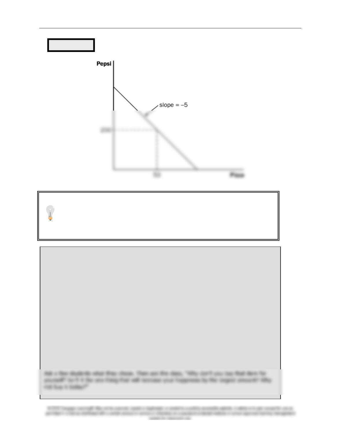
D. Using this information, we can draw the consumer’s budget constraint.
a. The slope of the budget constraint measures the rate at which the consumer can trade
one good for another.
b. The slope of the budget constraint equals the relative price of the two goods (1 pizza can
be traded for 5 liters of Pepsi).
This chapter is an advanced treatment of consumer choice using indifference curve
analysis. This chapter is much more difficult than the other chapters in the text. Most
undergraduate principles students will find this material challenging.
The best way to develop this model is to use specific examples with definite
quantities, prices, and levels of income.
Chapter 21/The Theory of Consumer Choice ❖ 347
Activity 1—You Can’t Always Get What You Want
Type: In-class activity
Topics: Budget constraints
Materials needed: None
Time: 5 minutes
Class limitations: Works in any size class
Purpose:
This activity shows consumers are restricted by their incomes and by the prices of goods.
Instructions:
Ask the students to think about maximizing their own utility. Specifically, ask them to assume
that billionaire Bill Gates offers to buy them the one thing that would increase their happiness
by the greatest amount. It cannot be money or a financial instrument, but he will buy them
any single thing they feel would make them happy. Have them write down their requested
item.
Figure 1
Although the book does it later, now might be a good time to show the effects of
price and income changes. Show mathematically and graphically how a doubling (or
halving) of the price of one good will cause its intercept to change. Also show what
happens to the vertical and horizontal intercepts when income changes. Emphasize
that the budget depicts the consumption possibilities available to the individual. The
consumer can be on or within the budget constraint, but not beyond it.

348 ❖ Chapter 21/The Theory of Consumer Choice
II. Preferences: What the Consumer Wants
A. Representing Preferences with Indifference Curves
1. A consumer is indifferent between two bundles of goods and services if the two bundles suit
her tastes equally well.
2. Definition of indifference curve: a curve that shows consumption bundles that give
the consumer the same level of satisfaction.
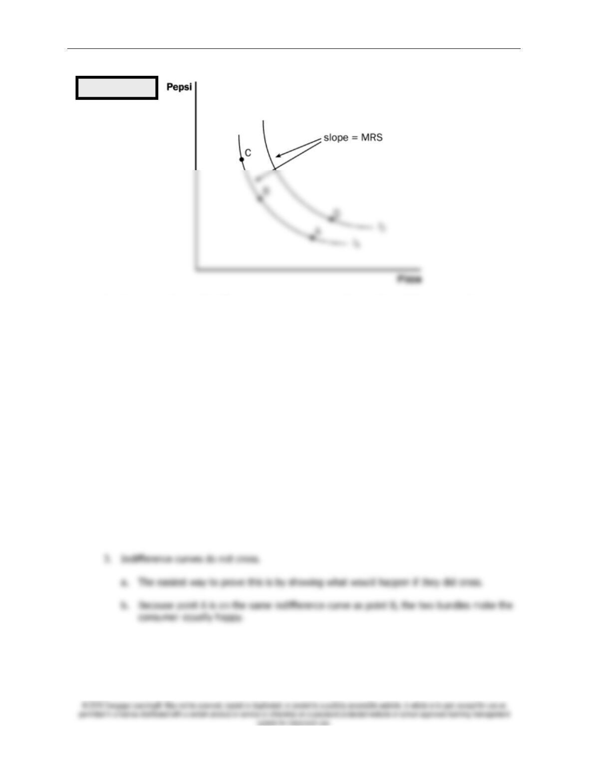
3. The consumer is indifferent among points A, B, and C.
5. The marginal rate of substitution is equal to the slope of the indifference curve at any point.
a. Because these indifference curves are not straight lines, the marginal rate of substitution
is not the same at all points on a given indifference curve.
The answer, of course, is they cannot afford it. Consumers’ purchases are constrained by
their incomes.
This eliminates the income barrier. Ask the class how many of them would spend the entire
amount of money buying that single good.
Some students would buy that item, but most would buy a variety of things. Using the money
for a single expensive item may not be the best way to allocate their newfound wealth.
Buying several cheap things may give a higher level of happiness.
Points for Discussion
1) Consumers have limited income.
2) Goods have prices.
Together these things determine the consumer’s budget constraint.
Chapter 21/The Theory of Consumer Choice ❖ 349
6. A consumer’s set of indifference curves gives a complete ranking of the consumer’s
preferences.
7. Any point on indifference curve
I
2 will be preferred to any point on indifference curve
I
1.
a. It is obvious that point D would be preferred to point A because point D contains more
pizza and more Pepsi.
b. We can tell, though, that point D is also preferred to point C because point D is on a
higher indifference curve.
B. Four Properties of Indifference Curves
1. Higher indifference curves are preferred to lower ones.
2. Indifference curves are downward sloping.
a. In most cases, the consumer would like more of both goods.
b. If the quantity of one good increases, the quantity of the other good must fall in order
for the consumer to remain equally satisfied.
Figure 2
350 ❖ Chapter 21/The Theory of Consumer Choice
c. Because point C is on the same indifference curve as point B, the two bundles make the
consumer equally happy.
d. But this should imply that points A and C make the consumer equally happy, even
though point C represents a bundle with more of both goods (which makes it preferred
to point A).
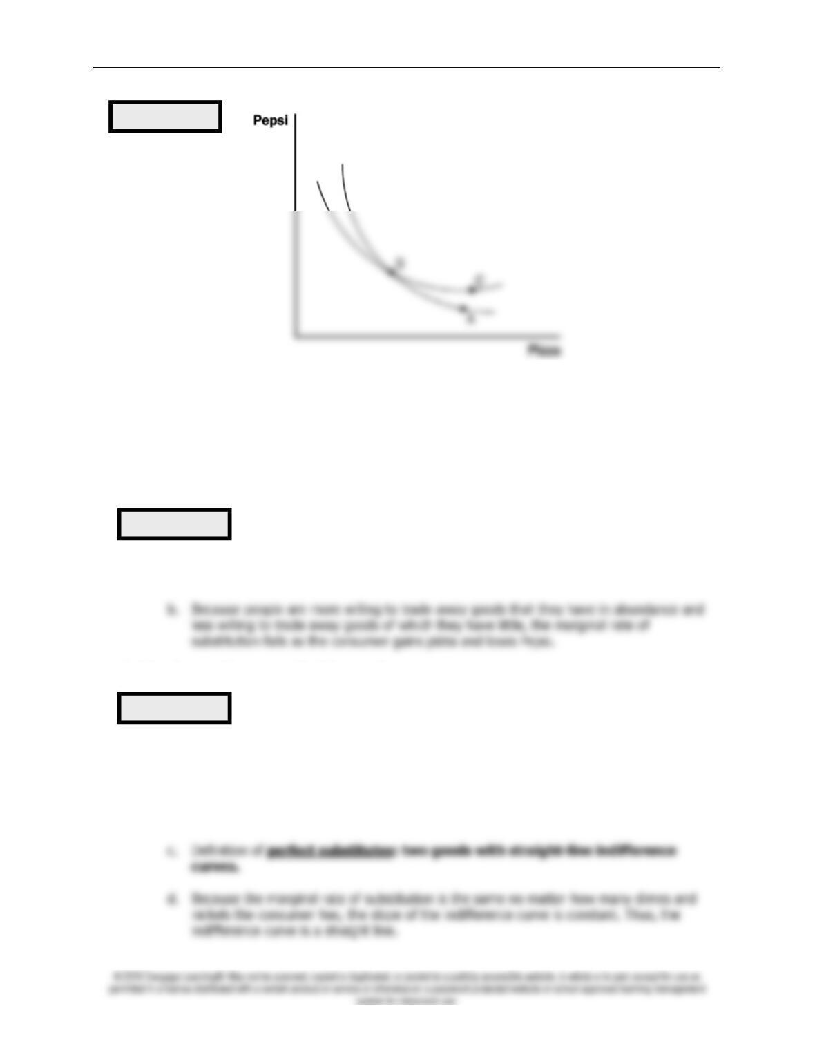
4. Indifference curves are bowed inward.
a. The slope of the indifference curve is the rate at which the consumer is willing to trade
one good for another.
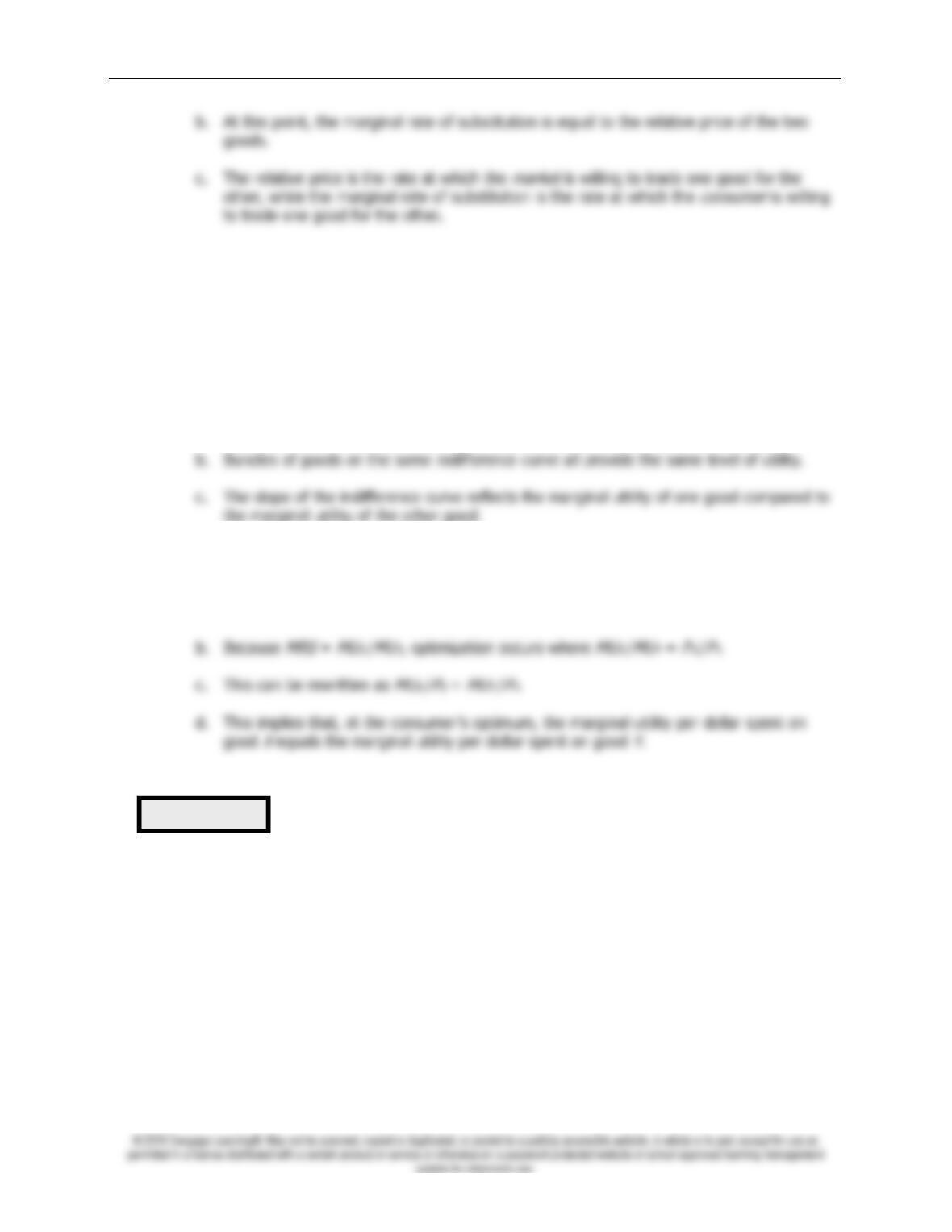
C. Two Extreme Examples of Indifference Curves
1. Perfect Substitutes
a. Examples: bundles of nickels and dimes.
b. Most likely, a consumer would always be willing to trade one dime for two nickels,
regardless of how many dimes or nickels she has.
Figure 3
Figure 4
Figure 5

Chapter 21/The Theory of Consumer Choice ❖ 351
2. Perfect Complements
a. Example: right shoes and left shoes.
b. Most likely, the consumer would only care about the number of
pairs
of shoes.
III. Optimization: What the Consumer Chooses
A. The Consumer’s Optimal Choices
1. The consumer would like to end up on the highest possible indifference curve, but she must
also stay within her budget.
2. The highest indifference curve the consumer can reach is the one that just barely touches
the budget constraint. The point where they touch is called the optimum.
3. The optimum point represents the best combination of Pepsi and pizza available to the
consumer.
4. At the optimum, the slope of the budget constraint is equal to the slope of the indifference
curve.
a. The indifference curve is tangent to the budget constraint at this point.
Figure 6
352 ❖ Chapter 21/The Theory of Consumer Choice
B.
FYI: Utility: An Alternative Way to Describe Preferences and Optimization
1. Utility is an abstract measure of the satisfaction that a consumer receives from a bundle of
goods and services.
2. A consumer will prefer bundle A to bundle B if bundle A provides more utility.
3. Indifference curves and utility are related.
a. Bundles of goods in higher indifference curves provide a higher level of utility.
4. A consumer can maximize her utility if she ends up on the highest indifference curve
possible.
a. This occurs when
MRS
=
PX
/
PY
.
C. How Changes in Income Affect the Consumer’s Choices
1. A change in income shifts the budget constraint.
a. An increase in income can be shown by an outward shift of the budget constraint; a
decrease in income means that the budget constraint shifts inward.
b. Because the relative price of the two goods has not changed, the slope of the budget
constraint remains the same.
2. An increase in income means that the consumer can now reach a higher indifference curve.
3. Because the consumer increased her consumption of both goods when her income increased,
both Pepsi and pizza must be normal goods.
Figure 7
Chapter 21/The Theory of Consumer Choice ❖ 353
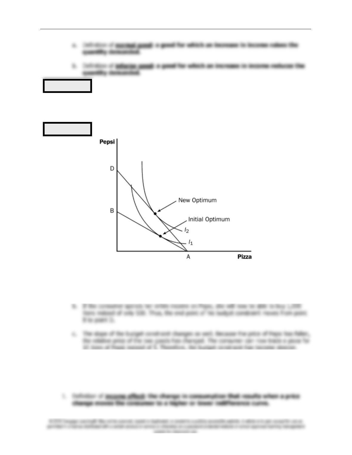
D. How Changes in Prices Affect the Consumer’s Choices
1. If the price of only one good changes, the budget constraint will have a different slope.
2. Suppose that the price of Pepsi falls from $2 per liter to $1.
a. If the consumer spends her entire income on pizza, the change in the price of Pepsi will
not affect her ability to buy pizza, so point A on the budget constraint remains the same.
3. How such a change in the price of one good alters the consumption of both goods depends
on the consumer’s preferences.
E. Income and Substitution Effects
Figure 8
Figure 9

354 ❖ Chapter 21/The Theory of Consumer Choice
2. Definition of substitution effect: the change in consumption that results when a
3. Suppose that the price of Pepsi falls.
a. The decrease in the price of Pepsi will make the consumer better off. Thus, if pizza and
Pepsi are both normal goods, the consumer will want to spread this improvement in her
purchasing power over both goods. This is the income effect and will make the consumer
want to buy more of both goods.
4. We can graphically decompose the change in the consumer’s decision into the income effect
and the substitution effect.
Figure 10
Students can learn to separate the substitution effects easily if they follow a simple
rule: Have them draw a line tangent to the original indifference curve but parallel to
the new budget constraint. Make sure that they realize that the substitution effect is
seen as the movement along one indifference curve (due to changes in relative
prices), and the income effect is seen as the movement from one budget constraint
to a parallel budget constraint (because the individual’s purchasing power has
changed).
Table 1
Chapter 21/The Theory of Consumer Choice ❖ 355
a. First, the consumer moves from the initial optimum (point A) to point B. The consumer is
equally happy at either of these points, but the marginal rate of substitution at point B
reflects the new relative prices of the two goods.
F. Deriving the Demand Curve
1. A demand curve shows how the price of a good affects the quantity demanded.
2. We can view a consumer’s demand curve as a summary of the optimal decisions that arise
from her budget constraint and indifference curves.
3. When the price of Pepsi falls from $2 per liter to $1, the consumer’s budget constraint shifts
4. Note that at a price of $2, the consumer’s quantity of Pepsi demanded is 50. At a price of $1,
quantity demanded is 150. These are two of the points on her demand curve for Pepsi.
IV. Three Applications
A. Do All Demand Curves Slope Downward?
1. The law of demand states that when the price of a good rises, people buy less of it.
2. However, it is possible that when the price of a good rises, people actually buy more of it.
3. Example: A consumer spends his entire budget on meat and potatoes. The price of potatoes
rises.
a. The budget constraint will shift in.
b. The substitution effect suggests that the consumer will choose more meat and fewer
potatoes.
Figure 11
Figure 12
356 ❖ Chapter 21/The Theory of Consumer Choice
dominates, the consumer will consume more potatoes even though the price of potatoes
rose.
4. Definition of Giffen good: a good for which an increase in the price raises the
quantity demanded.
5.
Case Study: The Search for Giffen Goods
B. How Do Wages Affect Labor Supply?
1. Example: Kayla has 100 hours per week that she can devote to working or enjoying leisure.
Her hourly wage is $50, which she spends on consumption goods.
2. We can show Kayla’s budget constraint graphically.
a. On the horizontal axis, we have hours of leisure. On the vertical axis, we have
consumption goods.
3. Kayla’s optimum will occur where the highest possible indifference curve is tangent to the
budget constraint.
4. If Kayla’s wage increases, her budget constraint will shift outward.
a. The budget constraint will become steeper, because Kayla can get more consumption for
every hour of leisure that she gives up.
b. We would expect that consumption would rise, because both the income and substitution
effects move in that direction. When the wage rises, leisure becomes relatively more
expensive. Thus, Kayla will increase consumption and decrease leisure. Also when Kayla’s
wage rises, her purchasing power is increased. Because consumption is a normal good,
Kayla will want more consumption.
Figure 13
Figure 14
Chapter 21/The Theory of Consumer Choice ❖ 357
d. If the substitution effect is greater than the income effect, Kayla will decrease leisure and
work more hours if her wage rises. This results in an upward-sloping labor supply curve.
5.
Case Study: Income Effects on Labor Supply: Historical Trends, Lottery Winners, and the
Carnegie Conjecture
a. One hundred years ago, workers worked six days a week. As wages (adjusted for
inflation) have risen, the length of the workweek has fallen. This suggests that a
backward-bending labor supply curve is not unrealistic.
C. How Do Interest Rates Affect Household Saving?
1. Example: Saul is planning ahead for retirement. There are two time periods. Currently, Saul
is young and working and able to earn a total income of $100,000. In the next period, Saul is
old and retired. He will have to consume using funds he saved while young. Assume that the
interest rate is 10 percent.
2. We can view “consumption while young” and “consumption while old” as the two goods that
Saul must choose between.
3. The interest rate determines the relative price of these two goods. For every dollar that Saul
saves while he is young, he can consume $1.10 when he is old.
4. We can draw Saul’s budget constraint.
a. On the horizontal axis, we have “consumption when young” and on the vertical axis, we
5. Saul’s optimum occurs where his highest possible indifference curve is tangent to his budget
constraint.
6. If the interest rate rises to 20 percent, two possible outcomes could occur.
Figure 15
Figure 16