Mishkin • Instructor’s Manual for The Economics of Money, Banking, and Financial Markets, Twelfth Edition 230
Chapter 21
ANSWERS TO QUESTIONS
1. When the inflation rate increases, what happens to the federal funds rate? Operationally,
how does the Fed adjust the federal funds rate?
2. What is the key assumption underlying the Fed’s ability to control the real interest rate?
3. Why does the MP curve necessarily have an upward slope?
The upward sloping MP curve implies that real interest rates rise, rather than fall, when
inflation increases. This is necessary because otherwise a rise in inflation would lead to a fall
4. If O = 0, what does this imply about the relationship between the nominal interest rate and
the inflation rate?
5. How does an autonomous tightening or easing of monetary policy by the Fed affect the MP
curve?
6. How is an autonomous tightening or easing of monetary policy different from a change in the
real interest rate caused by a change in the current inflation rate?
7. Suppose that a new Fed chair is appointed and that his or her approach to monetary policy
can be summarized by the following statement: “I care only about increasing employment.
Inflation has been at very low levels for quite some time; my priority is to ease monetary
policy to promote employment.” How would you expect the monetary policy curve to be
affected, if at all?
8. “The Fed decreased the fed funds rate in late 2007, even though inflation was increasing.
This action demonstrated a violation of the Taylor principle.” Is this statement true, false, or
uncertain? Explain your answer.
9. What factors affect the slope of the aggregate demand curve?
10. “Autonomous monetary policy is more effective at changing output when O is higher.” Is this
statement true, false, or uncertain? Explain your answer.
11. If net exports were not sensitive to changes in the real interest rate, would monetary policy
be more or less effective in changing output?
12. If an asset price bubble begins to form, assuming the central bank responds, how is it likely
to respond, and what will be the effect on the MP curve?
13. For each of the following situations, describe how (if at all) the IS, MP, and AD curves are
affected.
a. A decrease in financial frictions
The IS curve shifts to the right; the MP curve does not shift; the AD curve shifts to the
right.
b. An increase in taxes and an autonomous easing of monetary policy
The increase in taxes shifts the IS curve to the left, and the easing of monetary policy
moves the economy along the IS curve; the tax change does not affect the MP curve, but
c. An increase in the current inflation rate
An increase in the current inflation rate represents a movement along the MP curve,
d. A decrease in autonomous consumption
A decrease in autonomous consumption shifts the IS curve to the left; the MP curve does
e. Firms become more optimistic about the future of the economy.
f. The new Federal Reserve chair begins to care more about fighting inflation.
This represents an increase in O, which does not affect the IS curve; the MP curve
14. What would be the effect of an increase in U.S. net exports on the aggregate demand curve?
Would an increase in net exports affect the monetary policy curve? Explain.
An increase in U.S. net exports directly affects the IS curve, since planned expenditure
increases at every real interest rate. Assuming the goods market is in equilibrium, aggregate
15. Why does the aggregate demand curve shift when “animal spirits” change?
16. Suppose that government spending is increased at the same time that an autonomous
monetary policy tightening occurs. What will happen to the position of the aggregate demand
curve?
17. If financial frictions increase, how will this affect credit spreads, and how might the central
bank respond? Why?
The increase in financial frictions, if left alone, will increase the cost of borrowing and result
in higher credit spreads. This will lead to a decrease in planned investment, shifting the AD
curve to the left and reducing aggregate output demanded. Thus if the central bank wants to
18. “If
f
increases, then the Fed can keep output constant by reducing the real interest rate by
the same amount as the increase in financial frictions.” Is this statement true, false, or
uncertain? Explain your answer.
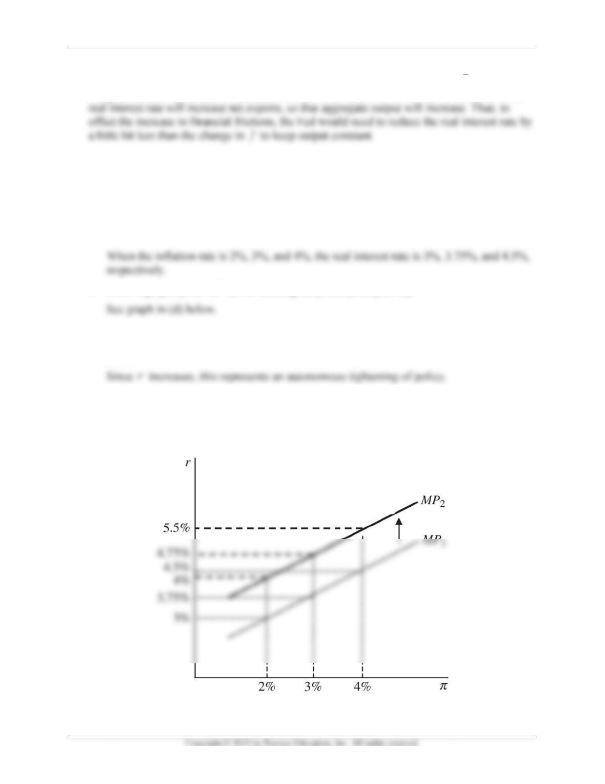
Mishkin •
Fals
e
miti
g
ANSW
E
19.
Assu
m
a.
C
b.
D
c.
A
m
p
d.
C
n
W
T
I
nstructor’s Ma
n
e
. If the Fed
c
g
ate the adv
e
E
RS TO AP
P
m
e that the
m
C
alculate th
e
D
raw a grap
h
A
ssume now
t
m
onetary po
l
o
licy?
C
alculate th
e
ew MP cur
v
W
hen the in
fl
T
he graph is
b
n
ual for The Ec
o
c
hanges int
e
e
rse effects o
P
LIED PR
O
m
onetary p
o
e
real intere
s
h
of the MP
t
hat the mo
n
l
icy curve re
p
e
real intere
s
v
e, showing
t
fl
ation rate i
s
b
elow.
o
nomics of Mon
e
e
rest rates b
y
f financial f
r
O
BLEMS
licy curve i
s
s
t rate when
curve, labe
l
n
etary polic
y
p
resent an
a
s
t rate when
t
he shift fro
m
s
2%, 3%, a
n
e
y, Banking, an
d
y
exactly th
e
r
ictions on i
n
s
given by r
=
the inflatio
n
l
ing the poin
y
curve is gi
v
a
utonomous
the inflatio
n
m
part (b).
n
d 4%, the r
e
d
Financial Mar
k
e
amount of
t
n
vestment.
H
=
1.5 + 0.7
5
n
rate is 2%,
ts from par
t
v
en by r = 2
.
tightening
o
n
rate is 2%,
e
al interest
r
k
ets, Twelfth E
d
t
he change i
n
H
owever, the
5
1
S
.
3%, and 4
%
t
(a).
.
5 + 0.751
S
.
o
r loosening
3%, and 4
%
r
ate is 4%, 4
d
ition
n
f,
this wi
l
e
decrease in
%
.
S
.
Does the n
e
of monetar
y
%
, and dra
w
.75%, and 5
234
l
l
the
e
w
y
w
the
.5%.
n
w
l
a
w
a
g
,
g
,
r
e
o
u
u
a
a
o
o
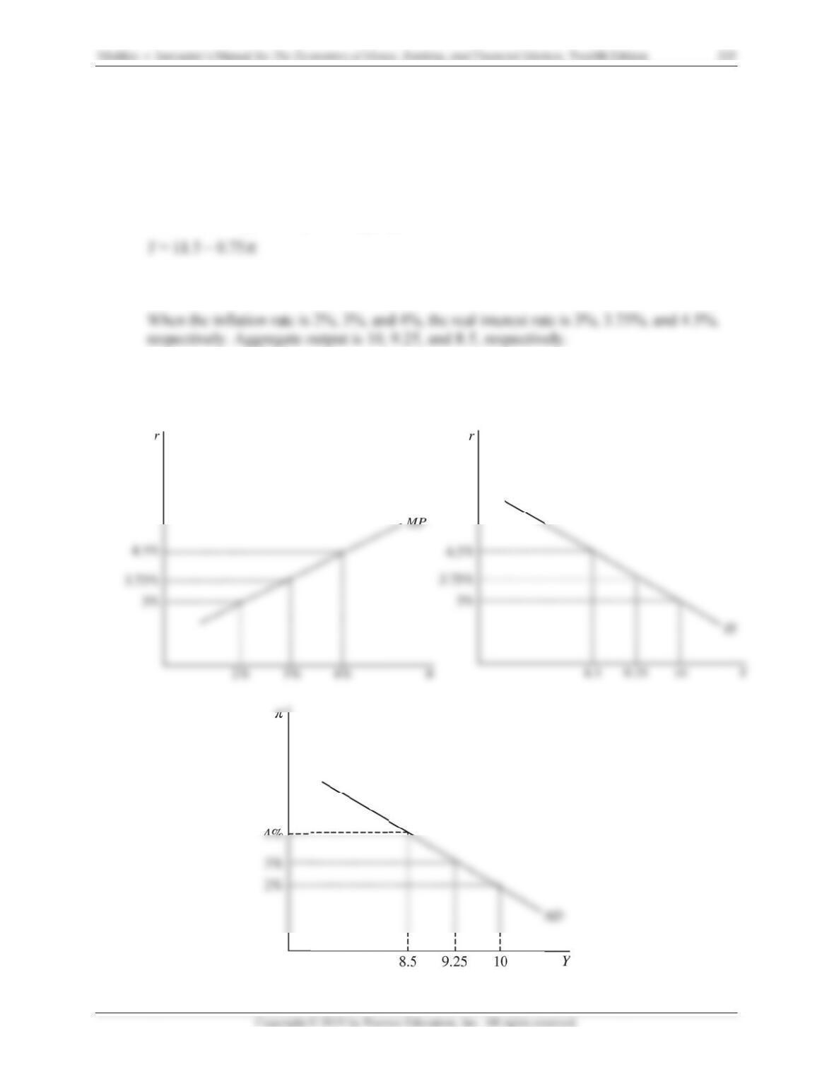
20.
Use
a
See
F
21.
Supp
o
Y =
1
a.
C
Y
Y
b.
C
a
n
c.
D
a
p
G
a
n IS curve
a
F
igure 4 in t
h
o
se the mon
e
1
3 – r.
C
alculate an
C
alculate the
n
d 4%.
D
raw graphs
p
propriate g
r
G
raphs are b
e
a
nd an MP
c
h
e textbook.
e
ta
r
y
policy
c
expression
fo
real interes
t
of the IS,
MP
r
aphs.
e
low.
c
urve to der
i
c
urve is giv
e
fo
r the aggre
g
t
rate and a
g
MP
, and AD c
i
ve graphic
a
e
n by r = 1.
5
g
ate deman
d
g
gregate out
p
urves, label
i
a
lly the AD
c
5
+ 0.751
S
,
a
d
curve.
p
ut when th
e
i
ng the poin
ts
c
urve.
a
nd the IS c
u
e
inflation r
a
t
s from part
(
u
rve is given
a
te is 2%, 3
%
(
b) on the
by
%
,
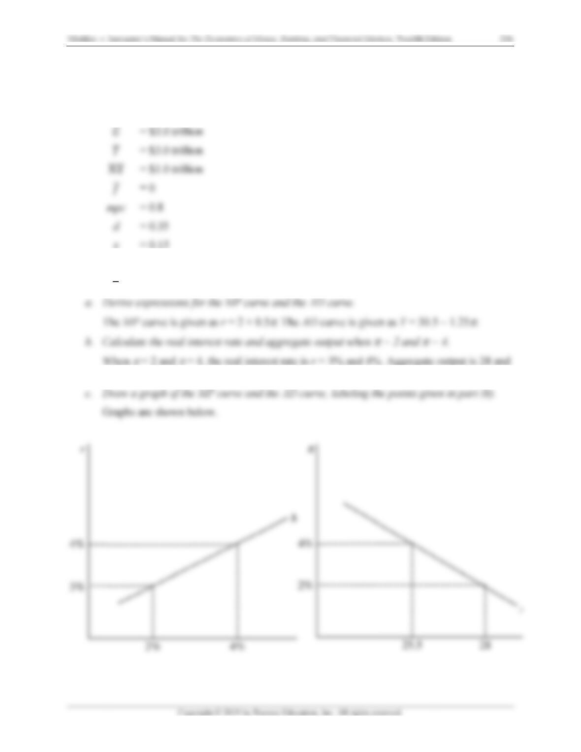
22.
Con
s
.
.
2
ider an eco
n
ܥ
ഥ
= $4
ܫ
ҧ
= $1
.
O
= 0.
5
r
= 2
5.5, respect
i
n
omy descri
b
trillio
n
.
5 trillion
5
i
vely.
b
ed by the f
o
o
llowing:
23. Consider an economy described by the following:
ܥ
ഥ = $3.25 trillion
ܫ
ҧ
= $1.3 trillion
ܰܺ
ത
ത
ത
ത
ത
= -$1.0 trillion
݂
ഥ= 1
mpc = 0.75
d = 0.3
a. Derive expressions for the MP curve and the AD curve.
b. Assume that
S
= 1. Calculate the real interest rate, the equilibrium level of output,
consumption, planned investment, and net exports.
c. Suppose the Fed increases r to r = 2. Calculate the real interest rate, the equilibrium
level of output, consumption, planned investment, and net exports at this new level of r.
d. Considering that output, consumption, planned investment, and net exports all decreased
in part (c), why might the Fed choose to increase r?
24. Consider the economy described in Applied Problem 23.
a. Derive expressions for the MP curve and the AD curve.
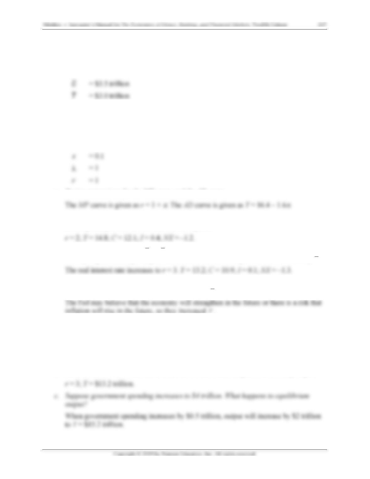
The MP curve is given as r = 1 +
S
. The AD curve is given as Y = 16.4 – 1.6
S
.
b. Assume that
S
= 2. What are the real interest rate and the equilibrium level of output?
Mishkin •
d.
If
m
25.
Supp
a.
D
S
Y
Y
b.
S
t
h
Y
c.
W
d
I
nstructor’s Ma
n
f
the Fed wa
m
ake?
o
se the MP
c
D
erive an ex
p
S
= 4, and
S
Su
ppose that
h
e new AD
c
Y
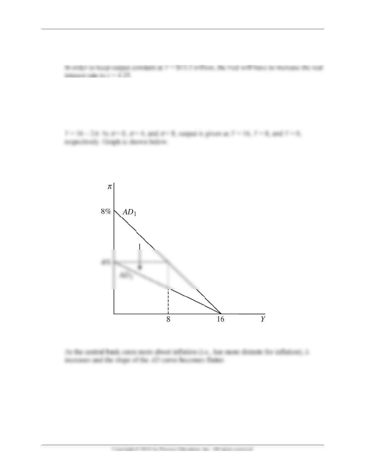
= 16 – 4
S
.
G
W
hat does y
o
d
istaste for i
n
n
ual for The Ec
o
nts to keep
o
c
urve is giv
e
p
ression for
S
= 8.
O
increases
c
urve using
t
G
raph is sh
o
o
ur answer t
o
n
flation and
o
nomics of Mon
e
o
utput const
a
e
n by r = 2
+
the AD cur
v
to
O
= 2. D
e
t
he graph fr
o
o
wn below,
w
o
part (b) i
m
the slope o
f
e
y, Banking, an
d
a
nt, then w
h
+
S
, and th
e
v
e, and dra
w
e
rive an exp
r
o
m part (a).
w
ith graph
fr
m
ply about t
h
f
the AD cur
v
d
Financial Mar
k
h
at monetar
y
e
IS curve is
w
a graph la
b
ression for
t
fr
om part (a)
h
e relations
h
v
e?
k
ets, Twelfth E
d
y
policy cha
n
given by Y
=
b
eling point
s
t
he new AD
c
.
h
ip between
d
ition
n
ge should i
t
=
20 – 2r.
s
at
S
= 0,
c
urve, and
d
a central b
a
238
t
d
raw
a
nk’s
Mishkin • Instructor’s Manual for The Economics of Money, Banking, and Financial Markets, Twelfth Edition 239
ANSWERS TO DATA ANALYSIS PROBLEMS
1. A measure of real interest rates can be approximated by the Treasury Inflation-Indexed
Security, or TIIS. Go to the St. Louis Federal Reserve FRED database and find data on the
five-year TIIS (FII5) and the personal consumption expenditure price index (PCECTPI), a
measure of the price index. Choose “Quarterly” for the frequency setting of the TIIS, and
download both data series. Convert the price index data to annualized inflation rates by
taking the quarter-to-quarter percent change in the price index and multiplying it by 4. Be
sure to multiply by 100 so that your results are percentages.
a. Calculate the average inflation rate and the average real interest rate over the most
recent four quarters of data available, and the four quarters prior to that.
b. Calculate the change in the average inflation rate between the most recent annual period
and the year prior. Then calculate the change in the average real interest rate over the
same period.
c. Using your answers to part (b), compute the ratio of the change in the average real
interest rate to the change in the average inflation rate. What does this ratio represent?
Comment on how it relates to the Taylor principle.
The ratio equals –1.05%/–0.28% = –0.3.74. This is an estimate of the coefficient Ȝ, which
2. A measure of real interest rates can be approximated by the Treasury Inflation-Indexed
Security, or TIIS. Go to the St. Louis Federal Reserve FRED database and find data on the
five-year TIIS (FII5) and the personal consumption expenditure price index (PCECTPI), a
measure of the price index. Choose “Quarterly” for the frequency setting for the TIIS, and
choose “Percent Change From Year Ago” for the units setting on (PCECTPI). Plot both
series on the same graph, using data from 2007 through the most current data available. Use
the graph to identify periods of autonomous monetary policy changes. Briefly explain your
reasoning.
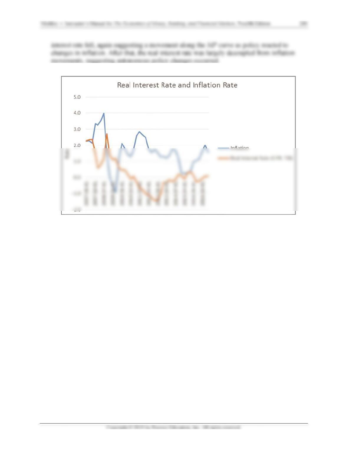
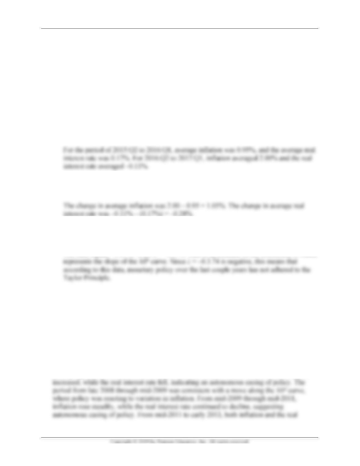
See graph below. Periods of autonomous monetary policy change are characterized by a
decoupling of real rates and inflation rates. From the middle of 2007 to late 2008, inflation