Basic Econometrics, Gujarati and Porter
CHAPTER 20:
SIMULTANEOUS-EQUATION METHODS
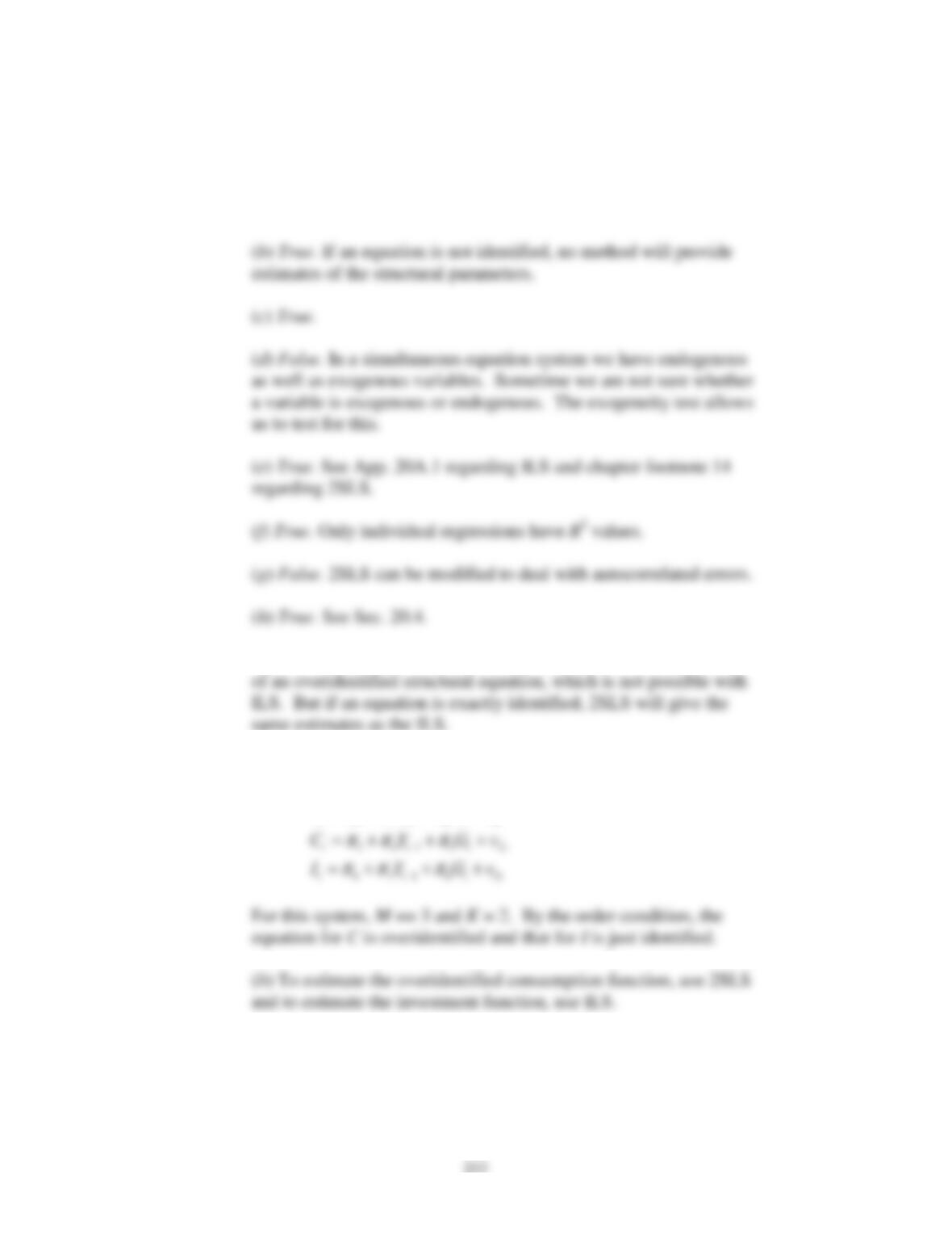
20.1 (a) False. OLS can be used in the recursive systems.
20.2 (a) 2SLS is designed to provide unique estimates of the parameters
20.3 (a) The three reduced form equations are:
0 1 1 2 1
t t t t
Y Y G v
π π π
−
= + + +
20.4 If the value of the R
2
in the first stage of 2SLS is high, it means that
the estimated values of the endogenous variables are very close to
their actual values; hence, the latter are less likely to be correlated
with the stochastic error term in the original structural equations. If,
Basic Econometrics, Gujarati and Porter
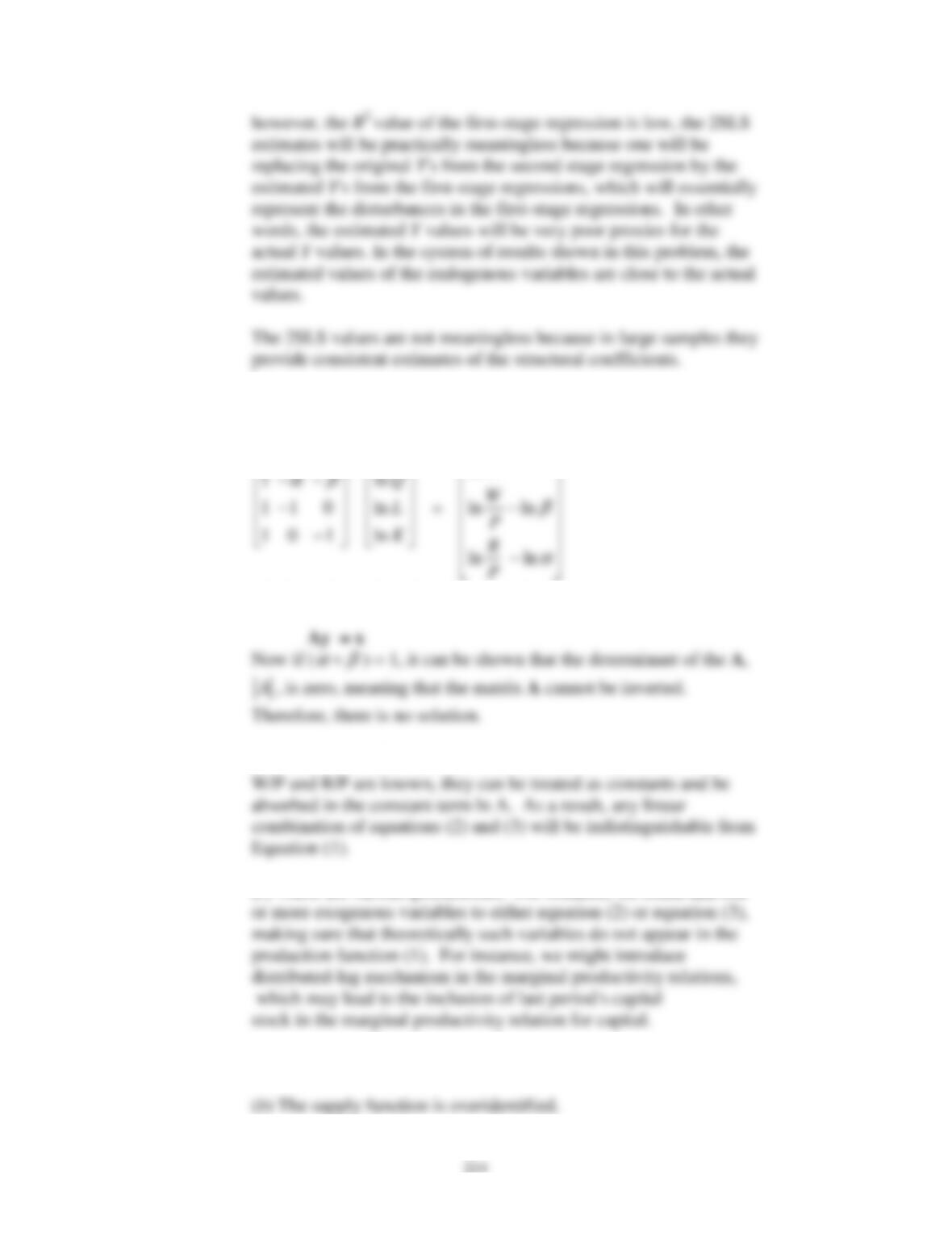
20.5 (a) Writing the system in matrix notation, we obtain:
ln
A
which can be written in matrix notation as:
(b) Even if
( ) 1
α β
+ ≠
, there is an identification problem. Since
(c
) There are various possibilities. For instance, we could add one
20.6
(
a
) The demand function is unidentified.
215
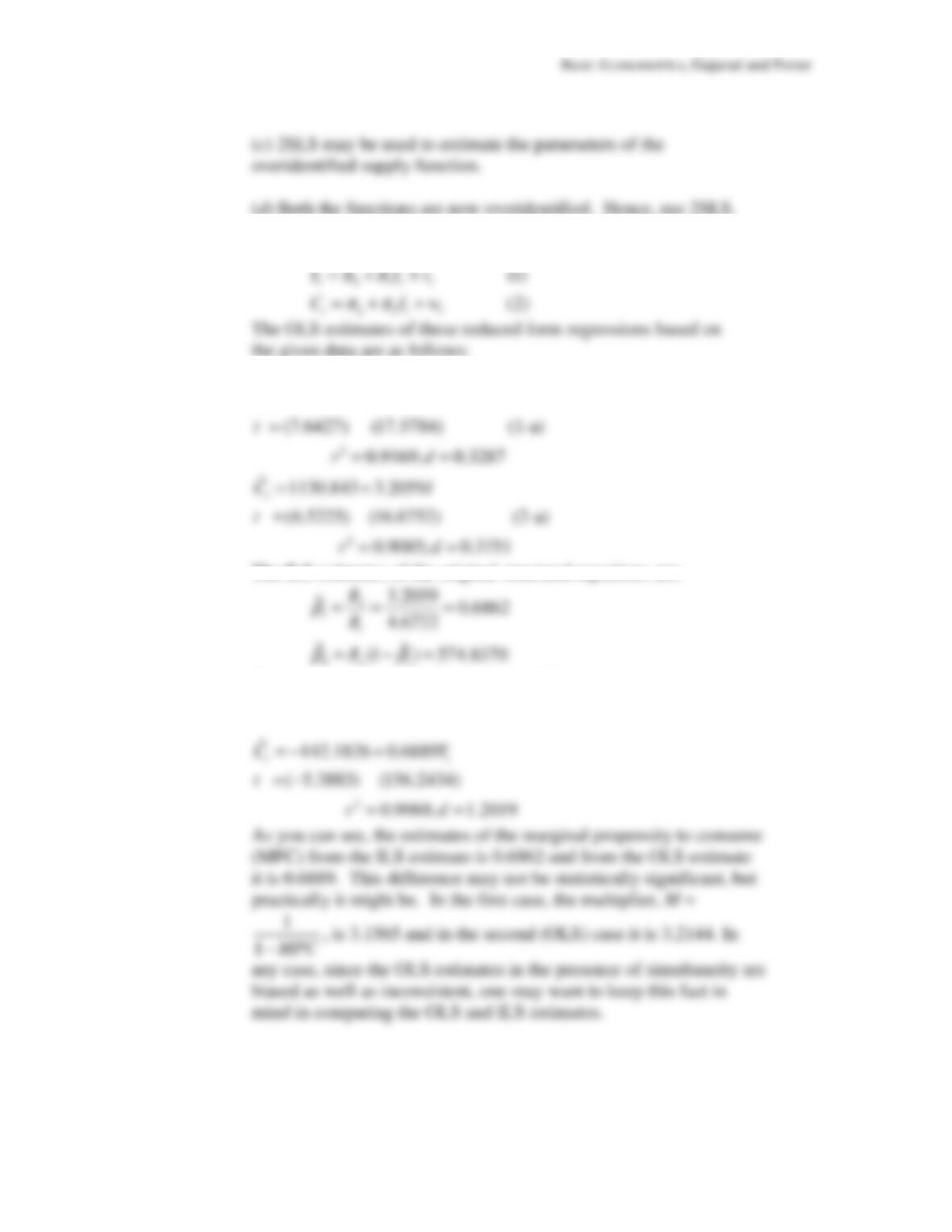
20.7
The reduced form equations are:
ˆ
1831.8580 4.6722
t t
Y I
= +
The ILS estimates of the original structural equations are:
For comparison, the OLS regression of C on Y gave the
following results:
Basic Econometrics, Gujarati and Porter
216
Empirical Exercises
20.8
(a) The IS-LM model of macroeconomics may be used to justify
this model.
20.9
(a) By the order condition, the interest rate equation is not
identified, and the income equation is overidentified.
20.10
Here both the equations are exactly identified. One can use ILS
or 2SLS to estimate the parameters, but they will give identical
results for reasons discussed in the chapter.
Basic Econometrics, Gujarati and Porter
217
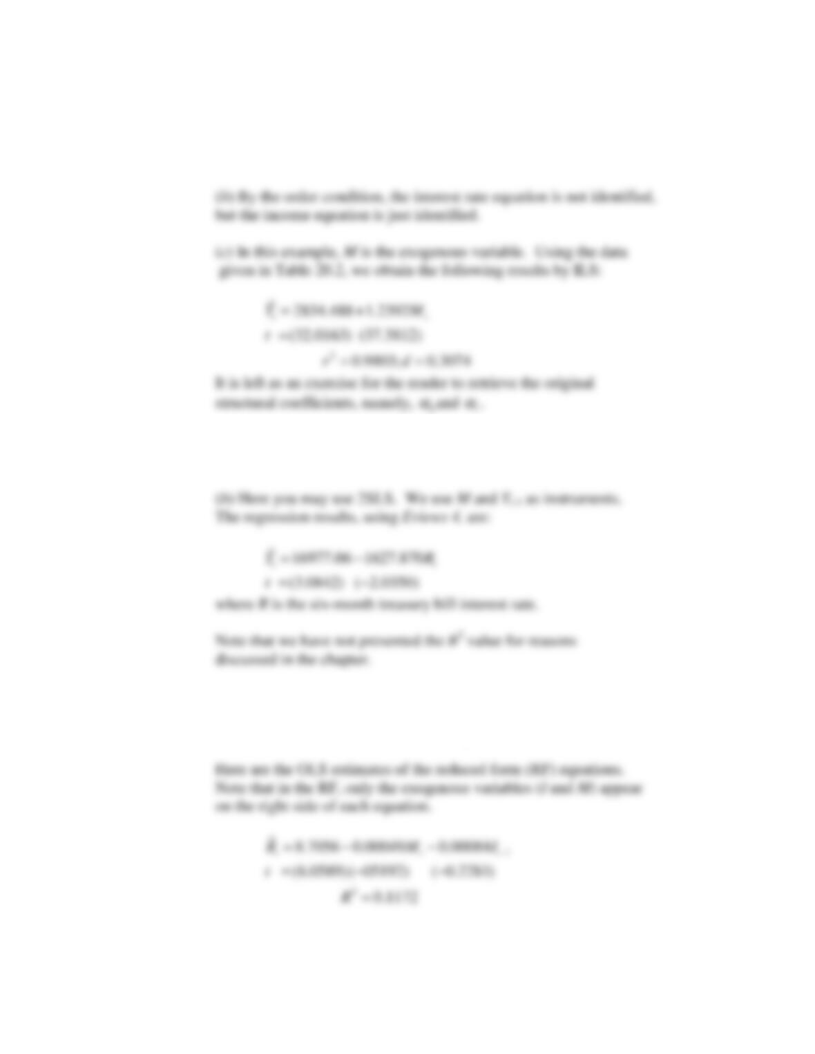
20.11
(a) Now the equations for R and Y are not identified, while
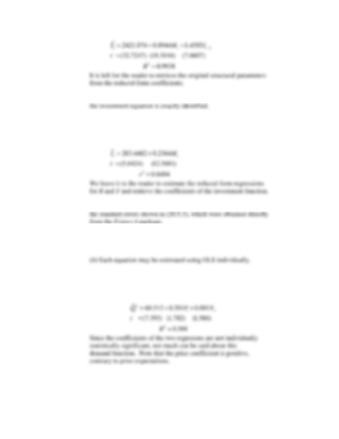
(b) First, we obtained the RF for the investment function. Since
there is only one exogenous variable, M, we regress I on M, which
gives the following results:
20.12
If you follow the procedure described in App.20A.2, you should get
20.13
(a) Since supply is a function of the price in the previous period,
the system is recursive. So, there is no simultaneity problem here.
(c) The regression results are as follows:
Demand Function:
Basic Econometrics, Gujarati and Porter
218
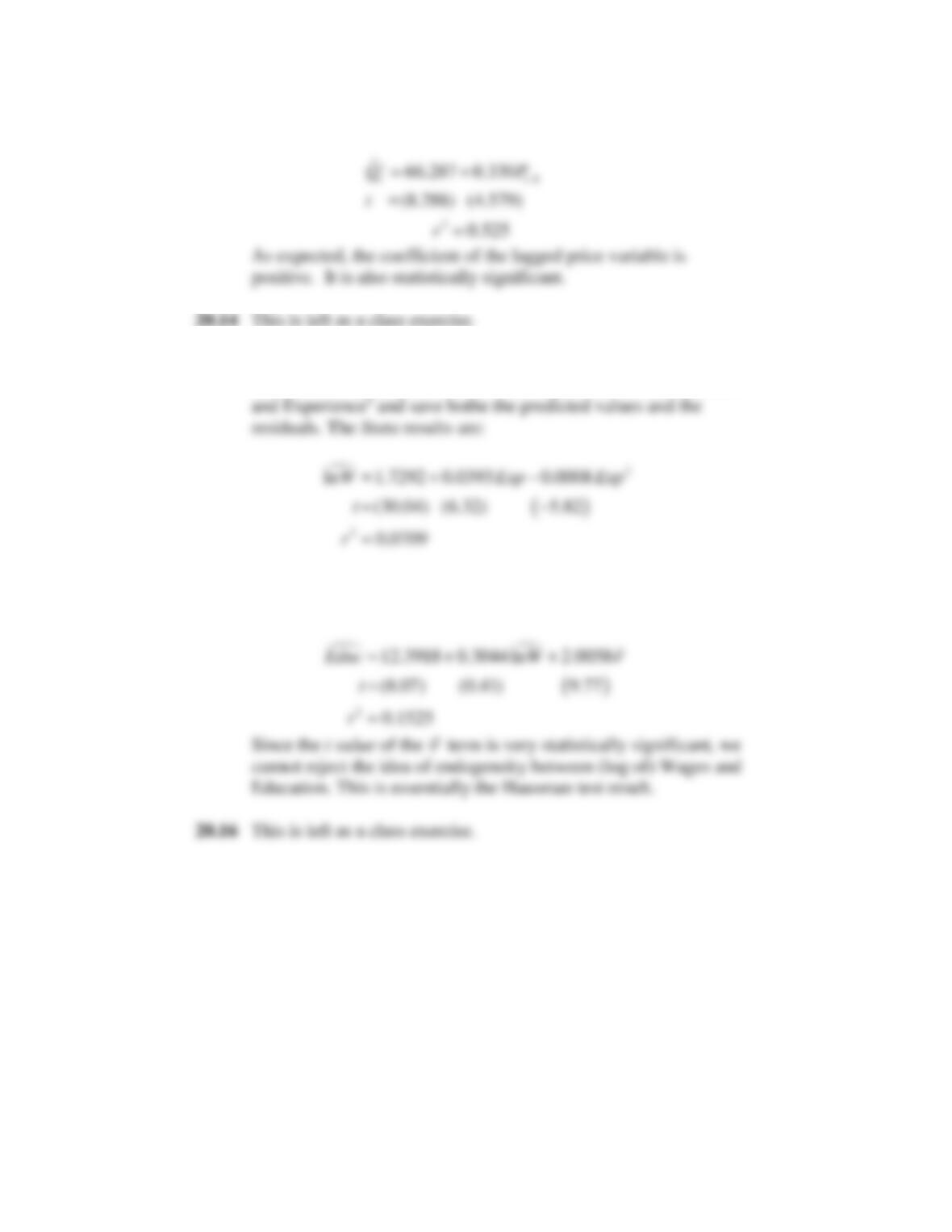
Supply Function
20.15
(a) and (b) One approach here is to follow the simultaneity testing
discussed in the chapter. First we will regress ln W on Experience
Now using the predcted ln W and residual values from above, we
create the following: