Chapter 20
Consumer Choice
◼ Overview
In this chapter, the classical theory of consumer choice using cardinal utility analysis is discussed. The
modern theory of consumer choice using indifference curve analysis is presented in the chapter appendix.
The classical approach assumes that people attempt to maximize their total utility subject to a budget
constraint. This early approach predicts how rational consumers will allocate their limited incomes so as
◼ Learning Objectives
After studying this chapter, students should be able to:
• 20.1 Distinguish between total utility and marginal utility and marginal utility and discuss why
marginal utility first rises but then declines
◼ Outline
I. Utility Theory: Utility is a term that economists use for satisfaction or want satisfying power of a
good or service. Utility is common to all goods that are desired. The concept of utility is purely
subjective; there is no way to measure the amount of utility that a consumer might be able to obtain
from a particular good. Utility does not mean “useful” or “utilitarian” or practical.
A. Tastes and Preferences and Utility: The utility that individuals receive from consuming a
good depends on their tastes and preferences.
1. Analyzing Utility: This chapter presents consumer decision making based on utility
maximization.
2. Utility and Utils: Economists first developed utility theory in terms of units of measurable
3. Total and Marginal Utility: Total utility is the amount of utility or satisfaction measured
4. Applying Marginal Analysis to Utility: The formula for marginal utility is this: Marginal
B. Graphical Analysis: A complete example is presented in Figure 20-1.
2. Negative Marginal Utility: When marginal utility is negative, an additional unit
C. Diminishing Marginal Utility (See Figure 20-1.)
1. The Law of Diminishing Marginal Utility: The principle that as more of any good or
II. Optimizing Consumption Choices: Consumer optimum is a choice of a set of goods and services
that maximizes the utility of each consumer, subject to limited income. This optimum is reached
when the marginal utility of the last dollar spent on each good yields the same utility and all income
is spent. (See Tables 20-1 and 20-2.)
A. A Two-Good Example: The rule of consumer optimum can be stated in algebraic terms by
B. A Two-Good Consumer Optimum: A complete numerical example is worked out in
Tables 20-1 and 20-2, which show that a consumer’s money income should be allocated so
C. A Little Math: The rule of consumer optimum can be stated in algebraic terms by examining
III. How a Price Change Affects Consumer Optimum
A. A Consumer’s Response to a Price Change (See Figure 20-2.)
1. A Price Change and the Consumer Optimum: Starting from the consumer optimum,
let the price of good A decrease. Consumers respond to the price decrease by consuming
B. The Substitution Effect: The substitution effect is the tendency of consumers to substitute
relatively cheaper goods for relatively more expensive ones.
1. An Example: If the relative price of a good falls, consumers will substitute in favor of this
2. Purchasing Power and Real Income: The real-income effect occurs when a change in
price causes a change in the purchasing power of a buyer’s income. A decrease in price
C. The Demand Curve Revisited: Linking the “law” of diminishing marginal utility and rule of
equal marginal utilities per dollar gives a negative relationship between the quantity demanded
of a good or service and its price. (See Figure 20-2.)
1. Marginal Utility, Total Utility, and the Diamond-Water Paradox: Although the total
utility of water is very high, water is much cheaper than diamonds, which have a much
lower total utility. (See Figure 20-3.)
a. Understanding the Paradox: This paradox is explained by the supply of water being
IV. Behavioral Economics and Consumer Choice Theory: Behavioral economists have doubts about
the rationality assumption, which causes them to question the utility-based theory of consumer
choice.
A. Does Behavioral Economics Better Predict Consumer Choices? The assumption of
B. Consumer Choice Theory Remains Alive and Well: Economists continue to assume that
◼ Points to Emphasize
Demand and Marginal Utility Analysis
The consumer is assumed to be rational and wants to maximize total utility subject to his or her budget
300 Miller • Economics Today, Nineteenth Edition
The Concept of Maximization Using Marginal Analysis
One of the keys to understanding maximization is the idea of marginal changes. Students have an
understanding that most decisions involve more or less and not either/or, but they have not usually put it
Utility Maximization
It should be understood why the ratio of the marginal utility of commodity one, divided by the price of
commodity one (i.e., MU1/P1), is equivalent to marginal utility per dollars worth for commodity one.
Assume that commodity one costs $1.00 per unit, and that the last unit consumed has a marginal utility
of 100 utils. Obviously, the marginal utility per dollar’s worth of expenditure on that commodity is 100
utils. Suppose price rises to $2.00 per unit. Now, because $2.00 still provides a marginal utility of 100
◼ For Those Who Wish to Stress Theory
The Algebra of Utility Maximization
Simple algebra will indicate that if MU1/Pl = MU2/P2 then MU1/MU2 = Pl/P2; both of these conditions are
true when the consumer is maximizing. What does MU1/MU2 = Pl/P2 mean? It says if the price of
commodity one is five times that of commodity two, then to be maximizing, the consumer must value
commodity one five times that of commodity two, on the margin. If P1/P2 MU1/MU2, then the consumer
Chapter 20 Consumer Choice 301
cannot be maximizing total utility; the consumer has consumed too much of commodity one, and not
enough of commodity two. Why? If Pl/P2 equals 4 to 1 and MU1/MU2 only 2 to 1, then this means that
The Indifference Curve and the Marginal Rate of Substitution
Those who wish to emphasize theory should discuss the appendix to this chapter. He or she will discover the
concept of the indifference curve and the marginal rate of substitution (the slope of the tangent to the
indifference curve). The shape of the indifference curve is discussed. It is convex with respect to the origin.
The meaning of higher and lower indifference curves is analyzed, along with consumer equilibrium. The latter
is found at the point of tangency of the budget line with an indifference curve. Indifference curve analysis is
then used to define normal and superior goods and to present the modern derivation of a demand curve.
302 Miller • Economics Today, Nineteenth Edition
◼ Further Questions for Class Discussion
1. It is fun to challenge students to try to think of any good, service, or activity that does not
eventually exhibit diminishing marginal utility per unit of time. You can easily refute their
2. It is instructive to ask your students how a rational consumer would allocate his or her
expenditures on goods and services if increasing marginal utility of goods was the general rule.
The first dollar of income would be spent on that good for which the marginal utility per dollar
3. Some Internet service providers have suggested that a way to deal with congestion on the Internet
is to charge customers for the use of bandwidth instead of simply charging a fixed price for an
unlimited amount of bandwidth use as is the case now. The idea is to provide a fixed amount
of bandwidth to each customer at a fixed rate. After the customer has used that bandwidth, each
additional unit of bandwidth used would have a price. What would be likely to happen to
downloads of high bandwidth videos and thus to congestion on the Internet? Explain in terms
4. When cell phones were first introduced, calls cost 10 cents per minute. Cell phones were first
used by consumers to get relatively important messages to another person, e.g., for emergencies.
Many people did not give out their cell phone numbers because receiving calls also cost 10 cents
per minute. How has cell phone use changed, and how is this change related to marginal utility
analysis? Most cell phone plans provide a large number of free minutes with the monthly fee. Some
5. In the healthcare reform law passed under the Obama administration, those who did not have
◼ Answers to Questions for Critical Analysis
Why a Consumer Optimum Can Include “Unlimited” Consumption in a
Pay-by-the-Minute Café (p. 442)
What fact ultimately constrains consumption of any item said to be available in “unlimited”
amounts at a fixed price? (Hint: Recall the law of diminishing marginal utility)
Monitoring the Provision of Legal Services to Ensure Attainment of a Consumer
Optimum (p. 444)
To ensure attainment of a consumer optimum, why might a client seek to ensure that the hourly
Do “Big–Box” Discount Retailers Contribute to Higher Obesity Rates among
Consumers? (pp. 446–447)
What happened to the marginal utility derived from food consumption as people responded to
◼ You Are There
Confronting the Challenge of Comparing Levels of Disutility from Pain (p. 449)
1. Why might two people diagnosed with exactly the same type of pain-inducing physical
problem opt to place different levels of daily stress on their bodies?
2. What does Michel’s experience imply about the idea of computing levels of utility derived
from consumption and contrasting these utilities across individuals? Explain.
304 Miller • Economics Today, Nineteenth Edition
◼ Issues and Applications
Two Different Utility Issues Associated with a “Pacemaker for the Stomach”
(pp. 449–450)
1. Explain why it must be true, even for someone trying to lose weight, that the last bite of
food consumed must have positive marginal utility at a consumer optimum?
2. What is true of the marginal utility per dollar spent on a stomach pacemaker compare with
◼ Research Project
◼ Appendix F—More Advanced Consumer Choice Theory
I. On Being Different: A difference curve is a curve composed of a set of consumption alternatives,
each of which yields the same total amount of satisfaction. (See Figure F-1.)
A. Properties of Indifference Curves:
1. Downward Slope: The indifference curve has a negative slope. (See Figure F-2.)
3. Imagining a Straight-Line Indifference Curve (See Figure F-2.)
II. The Budget Constraint and the Consumer Optimum: The budget constraint includes all of the
possible combinations of goods that can be purchased (at fixed prices) with a specific budget.
A. Slope of the Budget Constraint: The budget constraint is a line that slopes downward from left
to right. (See Figure F-5.)
III. Deriving the Demand Curve: The demand curve can be derived by changing the price of one good,
so that the budget line rotates. (See Figure F-7.)
Chapter 20 Consumer Choice 305
◼ Answers to Problems
20-1. The campus pizzeria sells a single pizza for $12. If you order a second pizza, however, the
pizzeria charges a price of only $5 for the additional pizza. Explain how an understanding
of marginal utility helps to explain the pizzeria’s pricing strategy.
The campus pizzeria indicates by its pricing policy that it recognizes the principle of diminishing
20-2. As an individual consumes more units of an item, the person eventually experiences
diminishing marginal utility. This means that to increase marginal utility, the person must
consume less of an item. Explain the logic of this behavior using the example in
Problem 20-1.
20-3. Where possible, complete the missing cells in the table below.
Number of
Cheeseburgers
Total Utility of
Cheeseburgers
Marginal
Utility of
Cheeseburgers
Bags of French
Fries
Total Utility of
French Fries
Marginal
Utility of
French Fries
0
0
—
0
0
—
1
20
—
1
—
10
2
36
—
2
—
8
3
—
12
3
—
2
4
—
8
4
21
—
5
—
4
5
21
—
The total utility of the third, fourth, and fifth cheeseburgers is 48, 56, and 60, respectively. The
20-4. From the data in Problem 20-3, if the price of a cheeseburger is $2, the price of a bag of
French fries is $1, and you have $6 to spend (and you spend all of it), what is the utility-
maximizing combination of cheeseburgers and French fries?
The utility-maximizing combination of cheeseburgers and bags of French fries that equates
20-5. Return to Problem 20-4. Suppose that the price of cheeseburgers falls to $1. Determine the
new utility-maximizing combination of cheeseburgers and French fries.
The new utility-maximizing combination of bags of French fries and cheeseburgers that equates
20-6. Suppose that you observe that total utility rises as more of an item is consumed. What can
you say for certain about marginal utility? Can you say for sure that it is rising or falling or
that it is positive or negative?
20-7. You determine that your daily consumption of soft drinks is 3 and your daily consumption
of tacos is 4 when the prices per unit are 50 cents and $1, respectively. Explain what
happens to your consumption bundle, and, after your consumption choices adjust, to the
marginal utility of soft drinks and the marginal utility of tacos, when the price of soft drinks
rises to 75 cents.
20-8. At a consumer optimum, for all goods purchased, marginal utility per dollar spent is
equalized. A high school student is deciding between attending Western State University
and Eastern State University. The student cannot attend both universities simultaneously.
Both are fine universities, but the reputation of Western is slightly higher, as is the tuition.
Use the rule of consumer optimum to explain how the student will go about deciding which
university to attend.
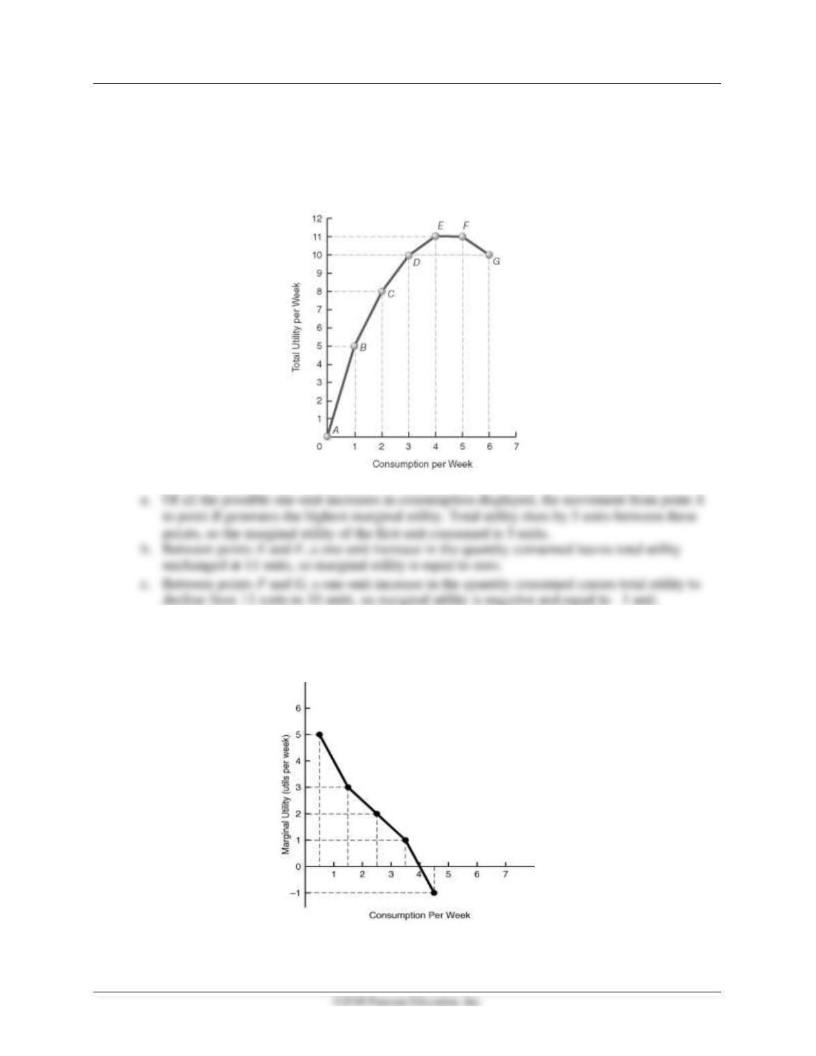
20-9. Consider the movements that take place from one point to the next (A to B to C and so on)
along the total utility curve at the next column as the individual successively increases
consumption by one more unit, and answer the questions that follow.
a. Which one-unit increase in consumption from one point to the next along the total
utility curve generates the highest marginal utility?
Chapter 20 Consumer Choice 307
b. Which one-unit increase in consumption from one point to the next along the total
utility curve generates zero marginal utility?
c. Which one-unit increase in consumption from one point to the next along the total
utility curve generates negative marginal utility?
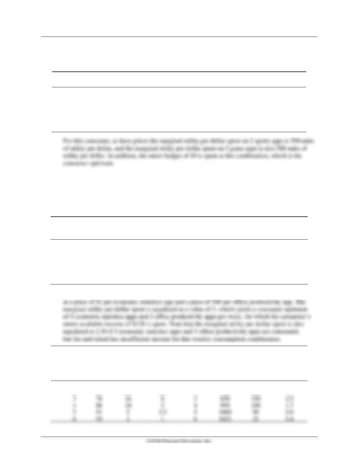
20-10. Draw a marginal utility curve corresponding to the total utility curve depicted in
Problem 20-9.
308 Miller • Economics Today, Nineteenth Edition
20-11. Refer to the table below. If the subscription price for a sports app is $2 per week, the
subscription price of a game app is $1 per week, and a student has $9 per week to spend,
what quantities will she purchase at a consumer optimum?
Quantity of Sports
Apps per week
Marginal Utility
(utils)
Quantity of Game
Apps per Week
Marginal Utility
(utils)
1
1,200
1
1,700
2
1,000
2
1,400
3
800
3
1,100
4
600
4
800
5
400
5
500
6
100
6
200
20-12. Refer to the following table for a different consumer, and assume that each year this
consumer buys only annual subscriptions to economics statistics apps and subscriptions to
office productivity apps. The price of a subscription to each type of economics statistics app
is $2 per year, and the price of a subscription to each office productivity app is $60 per year.
If the consumer’s available income is $128 per year, what quantity of each item will the
individual purchase each week at a consumer optimum?
Quantity of Subscriptions to
Economics Statistics Apps
per Year
Total Utility
(utils)
Quantity of Subscriptions
to Office Productivity Apps
per Week
Total Utility
(utils)
1
40
1
400
2
60
2
700
3
76
3
850
4
86
4
950
5
91
5
1,000
6
93
6
1,025
The table below displays the marginal utilities and the values of marginal utility per dollar spent
Quantity of
Hot Dogs per
Week
Total
Utility
Marginal
Utility
Marginal
Utility per
Dollar
Spent
Quantity
of
Baseball
Games
per Week
Total
Utility
Marginal
Utility
Marginal
Utility
per Dollar
Spent
1
40
—
—
1
400
—
—
2
60
20
10
2
700
300
5
4
86
10
4
950
100
5
91
5
5
6
93
2
6
20-13. In Problem 20-12, if the consumer’s income rises to $190 per week, what new quantities
characterize the new consumer optimum?
20-14. At a consumer optimum involving goods A and B, the marginal utility of good A is twice
the marginal utility of good B. The price of good B is $3.50. What is the price of good A?
20-15. At a consumer optimum involving goods X and Y, the marginal utility of good X equals
3 utils. The price of good Y is three times the price of good X. What is the marginal utility of
good Y?
20-16. At a consumer optimum involving goods A and B, the marginal utility of good A is 2 utils,
and the marginal utility of good B is 8 utils. How much greater or smaller is the price of
good B compared with the price of good A?
20-17. At a consumer optimum involving goods X and Y, the price of good X is $3 per unit, and the
price of good Y is $9 per unit. How much greater or smaller is the marginal utility of good
Y than the marginal utility of good X?
20-18. The marginal utility that an individual would experience if she were to consume the first
unit of a digital app is 15 utils, and the marginal utility that she would experience if she
were to consume a second unit is 18 utils. If one app is the amount that the individual
decides to consume, what is the person’s total utility?
20-19. Take a look at Figure 20-1. Suppose that the individual currently consumes 5 digital apps.
What happens to the person’s total utility if he were to reduce his consumption to 4 units?
Why does this fact imply that the marginal utility curve cuts through the horizontal axis of
panel (c) between the fourth and fifth app consumed?
20-20. Consider Figure 20-1. If this individual were to contemplate consuming a seventh digital
app and experience a total utility of 15 utils as a consequence, what would be the resulting
marginal utility? Would the points on the total utility and marginal utility graphs in panels
(a) and (b) lie higher and lower to the right of the current endpoints of those graphs?
20-21. Take a look at Table 20-1. Suppose that the price of each digital app falls to $3.30. At the
same time, the price of each portable power bank increases to $5.37. Income remains
unchanged at $26. Rework the marginal-utility-per-dollars-spent columns and round each
amount to the nearest one-tenth. What are the quantities of digital apps and portable power
banks now purchased by this consumer?
Total and Marginal Utility from Consuming Digital Apps and Portable Power Banks on an
Income of $26
(1)
(2)
(3)
(4)
(5)
(6)
(7)
(8)
Digital
Apps
per
Period
Total
Utility of
Digital
Apps per
Period
(utils)
Marginal
Utility
(utils)
MUd
Marginal
Utility per
Dollars
Spent
(MUd /Pd)
(price =
$5.97)
Portable
Power
Banks
per
Period
Total
Utility of
Portable
Power
Banks
per
Period
(utils)
Marginal
Utility
(utils)
MUp
Marginal
Utility per
Dollar Spent
(MUp /Pp)
(price =
$2.70)
0
0
–
–
0
0
–
–
1
50.0
50.0
8.4
1
25
25
9.3
2
95.0
45.0
5.0
2
47
22
8.1
3
40.0
6.7
3
65
18
6.7
4
36.5
7.8
4
80
15
5.6
5
28.5
8.6
5
89
3.3
20-22. At the optimal quantities of digital apps and portable power banks determined in your
answer to Problem 20-21, after rounding to the nearest 10 cents, is the $26 income all spent
at the new consumer optimum?
20-23. Consider figure 20-2, and suppose that the initial point is A. Explain why a decrease in the price
of each digital app from $5 to $4 results in a change in the marginal utilities of digital apps in a
direction that is consistent with re-attainment of a new consumer optimum at point B.
Appendix F
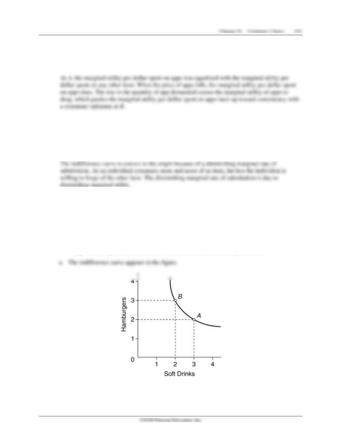
F-1. Consider the indifference curve illustrated in Figure F-1. Explain, in economic terms, why
the curve is convex to the origin.
F-2. Your classmate tells you that he is indifferent between three soft drinks and two
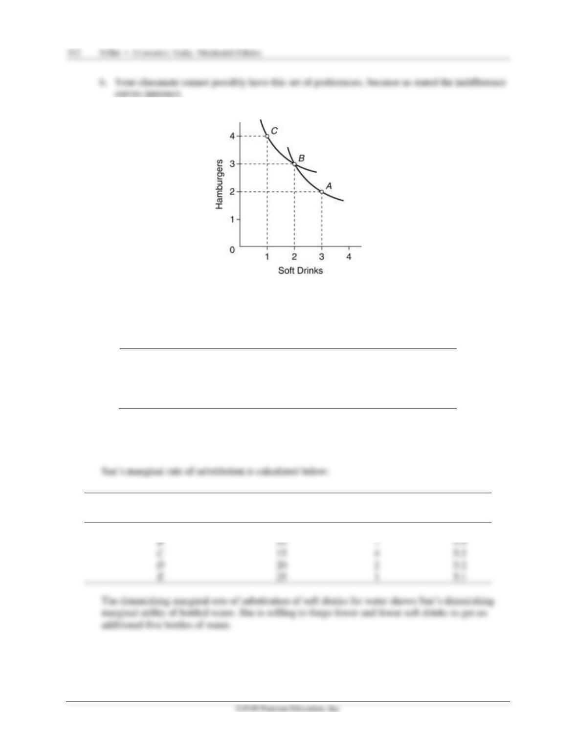
hamburgers or two soft drinks and three hamburgers.
a. Draw a rough diagram of an indifference curve containing your classmate’s
consumption choices.
b. Suppose that your classmate states that he is also indifferent between two soft drinks
and three hamburgers or one soft drink and four hamburgers, but that he prefers three
soft drinks and two hamburgers to one soft drink and four hamburgers. Use your
diagram from part (a) to reason out whether he can have these preferences.
F-3. The table below represents Sue’s preferences for bottled water and soft drinks, the
combination of which yields the same level of utility.
Combination of Bottled Water
and Soft Drinks
Bottled Water per
Month
Soft Drinks per
Month
A
5
11
B
10
7
C
15
4
D
20
2
E
25
1
Calculate Sue’s marginal rate of substitution of soft drinks for bottled water at each rate of
consumption of water (or soft drinks). Relate the marginal rate of substitution to marginal
utility.
Combination of Bottled
Water and Soft Drinks
Bottled Water per
Month
Soft Drinks per
Month
MRS
A
5
11
C
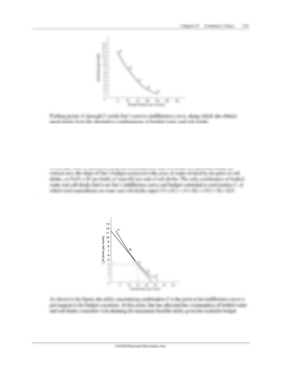
F-4. Using the information provided in Problem F-3, illustrate Sue’s indifference curve, with
water on the horizontal axis and soft drinks on the vertical axis.
F-5. Sue’s monthly budget for bottled water and soft drinks is $23. The price of bottled water is
$1 per bottle, and the price of soft drinks is $2 per bottle. Calculate the slope of Sue’s
budget constraint. Given this information and the information provided in Problem F-3,
find the combination of goods that satisfies Sue’s utility maximization problem in light of
her budget constraint.
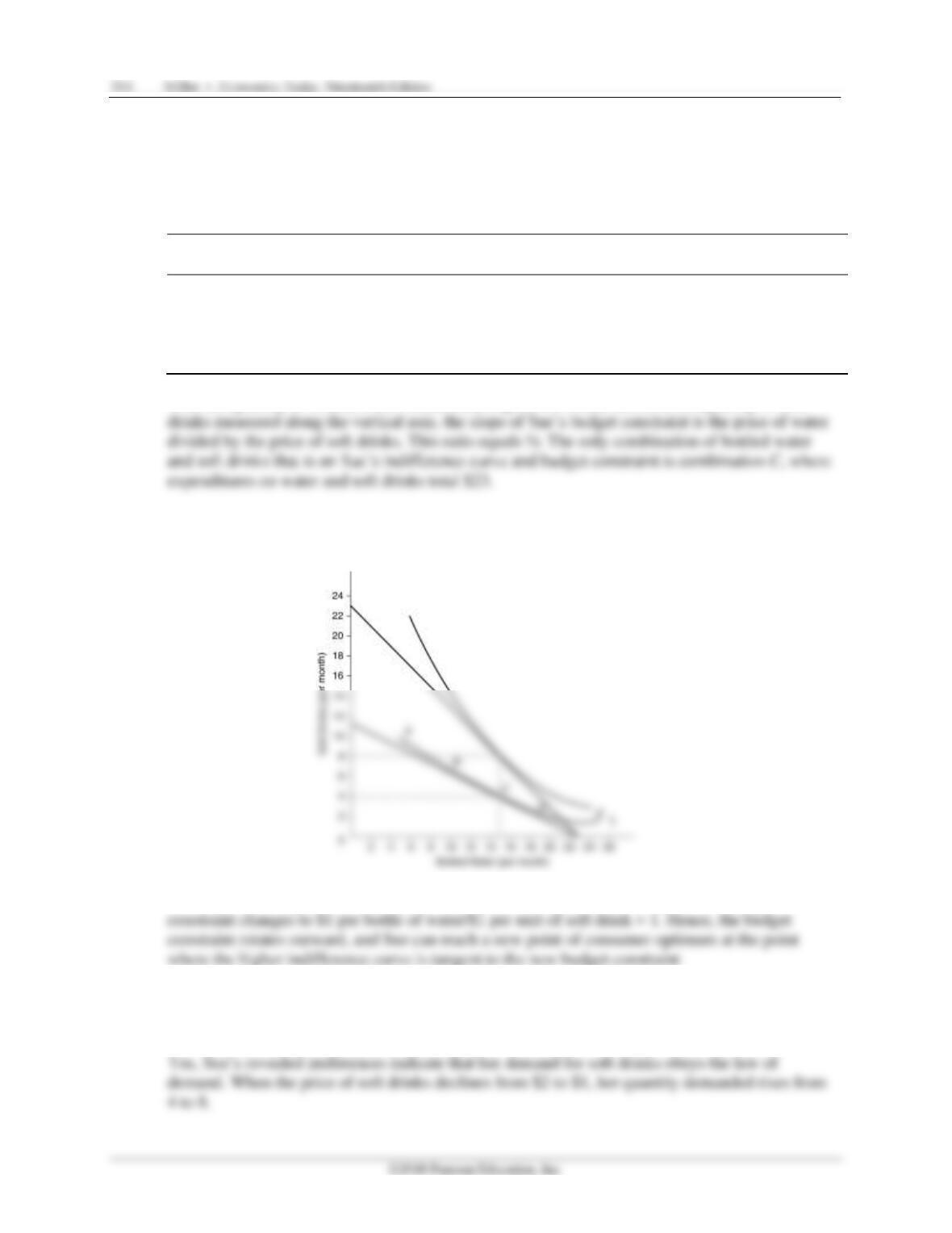
F-6. Using the indifference curve diagram you constructed in Problem F-4, add in Sue’s budget
constraint using the information in Problem F-5. Illustrate the utility-maximizing
combination of bottled water and soft drinks.
F-7. Suppose that at a higher satisfaction level than in Problem F-3, Sue’s constant-utility
preferences are as shown in the table below. Calculate the slope of Sue’s new budget
constraint using the information provided in Problem F-5. Supposing now that the
price of a soft drink falls to $1, find the combination of goods that satisfies Sue’s
utility maximization problem in light of her budget constraint.
Combination of Bottled
Water and Soft Drinks
Bottled Water per Month
Soft Drinks per Month
A
5
22
B
10
14
C
15
8
D
20
4
E
25
2
With the quantity of bottled water measured along the horizontal axis and the quantity of soft
F-8. Illustrate Sue’s new budget constraint and indifference curve in a diagram from the data in
Problem F-3. Illustrate also the utility-maximizing combination of goods.
As shown in the figure, when the price of soft drinks drops to $1, the slope of the budget
F-9. Given your answers to Problems F-5 and F-7, are Sue’s preferences for soft drinks
consistent with the law of demand?
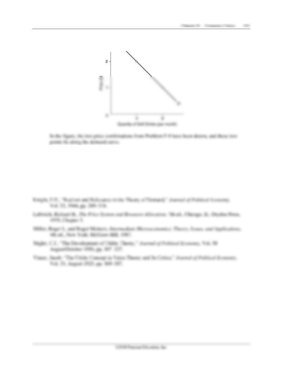
F-10. Using your answer to Problem F-8, draw Sue’s demand curve for soft drinks.
◼ Selected References
Ferguson, C.W., “Substitution Effect in Value Theory: A Pedagogical Note,” Southern Economic
Journal, Vol. XXVI, 1960, pp. 310–314.
Fisher, Irving, “Is ‘Utility’ the Most Suitable Term for the Concept It Is Used to Denote?” American
Economic Review, Vol. 8, June 1918, pp. 335–337.