
32
CASE STUDY EXTENSION
2-4 The Components of GDP
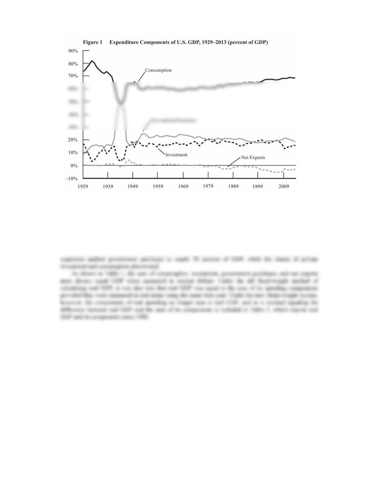
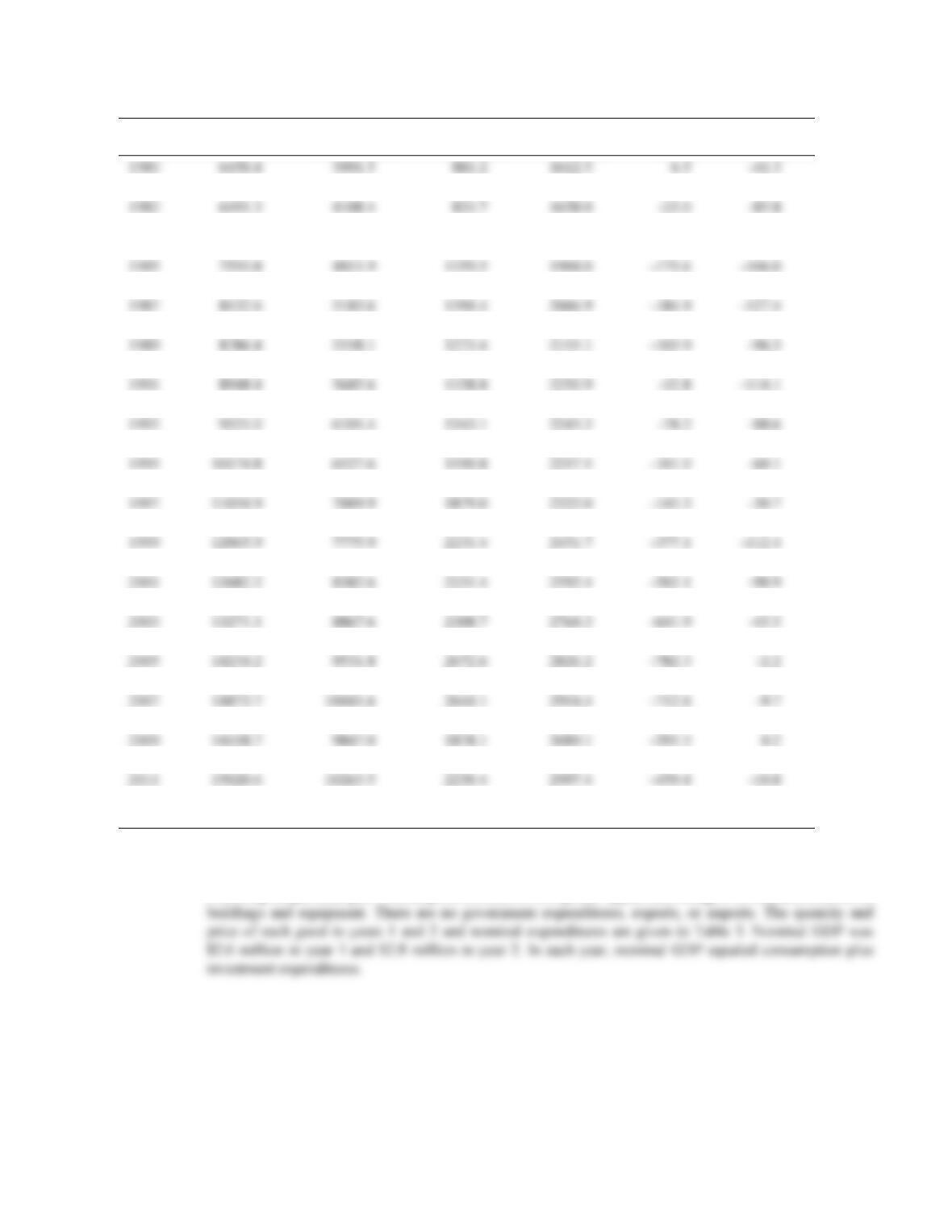
Table 1 and Figure 1 show the principal components of GDP between 1929 and 2013.
Table 1 U.S. Nominal GDP and the Components of Expenditure: 1929–2013 (billions of dollars)
Year
GDP
Consumption
Investment
Government
Purchases
Net
Exports
1929
104.6
77.4
17.2
9.6
0.4
1931
77.4
60.7
6.5
10.2
0.0
1932
59.5
48.7
1.8
9.0
0.0
1933
57.2
45.9
2.3
8.9
0.1
1934
66.8
51.5
4.3
10.7
0.3
1935
74.3
55.9
7.4
11.2
–0.2
1936
84.9
62.2
9.4
13.4
–0.1
1937
93.0
66.8
13.0
13.1
0.1
1938
87.4
64.3
7.9
14.2
1.0
1939
93.5
67.2
10.2
15.2
0.8
1940
102.9
71.3
14.6
15.6
1.5
1941
129.4
81.1
19.4
27.9
1.0
1942
166.0
89.0
11.8
65.5
–0.3
1943
203.1
99.9
7.4
98.1
–2.2
1944
224.6
108.6
9.2
108.7
1945
228.2
120.0
12.4
96.6
–0.8
1946
227.8
144.3
33.1
43.2
7.2
1947
249.9
162.0
37.1
40.0
10.8
1948
274.8
175.0
50.3
44.0
5.5
1949
272.8
178.5
39.1
50.0
5.2
1950
300.2
192.2
56.5
50.7
0.7
1951
347.3
208.5
62.8
73.5
2.5
1952
367.7
219.5
57.3
89.8
1.2
1953
389.7
233.0
60.4
97.0
–0.7
1954
391.1
239.9
58.1
92.8
0.4
1955
426.2
258.7
73.8
93.3
0.5
1956
450.1
271.6
77.7
98.5
2.4
1957
474.9
286.7
76.5
107.5
4.1
1958
482.0
296.0
70.9
114.5
0.5
1959
522.5
317.5
85.7
118.9
0.4
1960
543.3
331.6
86.5
121.0
4.2
1961
563.3
342.0
86.6
129.8
4.9
1962
605.1
363.1
97.0
140.9
4.1
1963
638.6
382.5
103.3
147.9
4.9
1964
685.8
411.2
112.2
155.5
6.9
1965
743.7
443.6
129.6
164.9
5.6
1966
815.0
480.6
144.2
186.4
3.9
1967
861.7
507.4
142.7
208.1
3.6
1968
942.5
557.4
1.4
1969
1019.9
604.5
173.6
240.4
1.4
1970
1075.9
647.7
170.1
254.2
4.0
1971
1167.8
701.0
196.8
169.3
0.6
1930
92.2
70.1
11.4
10.3
0.3

33
Table 1 U.S. Nominal GDP and the Components of Expenditure: 1929–2010 (billions of dollars)
(continued)
Year
GDP
Consumption
Investment
Government
Purchases
Net
Exports
1972
1282.4
769.4
228.1
288.2
–3.4
1974
1548.8
932.0
274.5
343.1
–0.8
1975
1688.9
1032.8
257.3
382.9
1976
1877.6
1150.2
323.2
405.8
–1.6
1977
2086.0
1276.7
396.6
435.8
–23.1
1978
2356.6
1426.2
478.4
477.4
–25.4
1979
2632.1
1589.5
539.7
525.5
–22.5
1980
2862.5
1754.6
530.1
590.8
–13.1
1981
3211.0
1937.5
631.2
654.7
–12.5
1982
3345.0
2073.9
581.0
710.0
–20.0
1983
3638.1
2286.5
637.5
765.7
–51.6
1984
4040.7
2498.2
820.1
825.2
–102.7
1985
4346.7
2722.7
829.6
908.4
–114
1986
4590.2
2898.4
849.1
974.5
–131.9
1987
4870.2
3092.1
892.2
1030.8
–144.8
1988
5252.6
3346.9
937.0
1078.2
–109.4
1989
5657.7
3592.8
999.7
1151.9
–86.7
1990
5979.6
3825.6
993.5
1238.4
–77.9
1991
6174.0
3960.2
944.3
–28.6
1992
6539.3
4215.7
1013.0
1345.4
–34.7
1993
6878.7
4471.0
1106.8
1366.1
–65.2
1994
7308.8
4741.0
1256.5
1403.7
–92.5
1995
7664.1
4984.2
1317.5
1452.2
–89.8
1996
8100.2
5268.1
1432.1
1496.4
–96.4
1997
8608.5
5560.7
1595.6
1554.2
–102.0
1998
9089.2
5903.0
1735.3
1613.5
–162.7
1999
9660.6
6307.0
1726.0
–256.6
2000
10284.8
6792.4
2033.8
1834.4
–375.8
2001
10621.8
7103.1
1928.6
1958.8
–368.7
2002
10977.5
7384.1
1925.0
2094.9
–426.5
2003
11510.7
7765.5
2027.9
2220.8
–503.7
2004
12274.9
8260.0
2276.7
2357.4
–619.2
2005
13093.7
8794.1
2527.1
2493.7
–721.2
2006
13855.9
9304.0
2680.6
2642.2
–770.9
2007
14477.6
9750.5
2643.7
2801.9
–718.5
2008
14718.6
10013.6
2424.8
3003.2
–723.1
2009
14418.7
9847.0
1878.1
3089.1
–395.4
2010
14964.4
10202.2
2100.8
3174.0
–512.7
2011
15517.9
10689.3
2239.9
3168.7
–580.0
2012
16163.2
11083.1
2479.2
3169.2
–568.3
2013
16768.1
11484.3
2648.0
3143.9
–508.2
Source: U.S. Department of Commerce, Bureau of Economic Analysis.
1973
1428.5
851.1
266.9
306.4
34
Source: U.S. Department of Commerce, Bureau of Economic Analysis. Data are expressed as a percentage of
GDP.
As Figure 1 illustrates, the GDP shares of consumption expenditure, private investment expenditure,
and government purchases have been relatively constant over the past 60 years. Earlier in the twentieth
century, however, the story was much different as expenditure shares shifted sharply. During the Great
Depression of the early 1930s, the collapse of investment spending led to a decline in its share of GDP
while the share of consumption expenditure increased. During World War II, the federal government’s
35
Table 2 U.S. Real GDP and the Components of Expenditure: 1980–2013 (billions of chained 2009 dollars)
Year
GDP
Consumption
Investment
Government
Purchases
Net
Exports
Residual
1981
6617.7
4050.8
958.7
1628.0
1.3
–21.1
1982
6491.3
4108.4
833.7
1658.0
–23.0
–85.8
1983
6792.0
4342.6
911.5
1721.6
–79.2
–104.5
1984
7285
4571.6
1160.3
1783.2
–154.0
–76.1
1985
7593.8
4811.9
1159.5
1904.0
–106.0
1986
7860.5
5014.0
1161.3
2007.7
–193.9
–128.6
1987
8132.6
5183.6
1194.4
2066.9
–184.9
–127.4
1988
8474.5
5400.5
1223.8
2094.8
–136.0
–108.6
1989
8786.4
5558.1
1273.4
2155.1
–103.9
–96.3
1990
8955.0
5672.6
1240.6
2224.3
–76.5
–106.0
1991
8948.4
5685.6
1158.8
2250.9
–32.8
–114.1
1992
9266.6
5896.5
1243.7
2262.1
–35.7
–100.0
1993
9521.0
6101.4
1343.1
2243.3
–78.2
–88.6
1994
9905.4
6338.0
1502.3
2245.5
–111.0
–69.4
1995
10174.8
6527.6
1550.8
2257.5
–101.0
–60.1
1996
10561.0
6755.6
1686.7
2279.2
–114.6
–45.9
1997
11034.9
7009.9
1879.0
2322.0
–145.3
–30.7
1998
11525.9
7384.7
2058.3
2370.5
–265.5
–22.1
1999
12065.9
7775.9
2231.4
2451.7
–377.1
–112.4
2000
12559.7
8170.7
2375.5
2498.2
–477.8
–83.6
2001
12682.2
8382.6
2231.4
2592.4
–502.1
–90.9
2002
12908.8
8598.8
2218.2
2705.8
–584.3
–70.5
2003
13271.1
8867.6
2308.7
2764.3
–641.9
–45.5
2004
13773.5
9208.2
2511.3
2808.2
–734.7
–19.6
2005
14234.2
9531.8
2672.6
2826.2
–782.3
–2.2
2006
14613.8
9821.7
2730.0
2869.3
–794.2
–3.8
2007
14873.7
10041.6
2644.1
2914.4
–712.6
–9.7
2008
14830.4
10007.2
2396
2994.8
–557.8
–13.6
2009
14418.7
9847.0
1878.1
3089.1
–395.5
2010
14783.8
10036.3
2120.4
3091.4
–458.8
–1.1
2011
15020.6
10263.5
2230.4
2997.4
–459.4
–10.8
2012
15369.2
10449.7
2435.9
2953.9
–452.5
–17.3
2013
15710.3
10699.7
2556.2
2894.5
–420.5
–22.5
Source: U.S. Department of Commerce, Bureau of Economic Analysis.
To understand why a chain–weight method violates the identity Y = C + I + G + NX, consider the
following simple example. Consumption consists of two goods: apples and oranges. Investment consists of
6450.4
3991.5
881.2
1612.5
6.5
–41.3
36
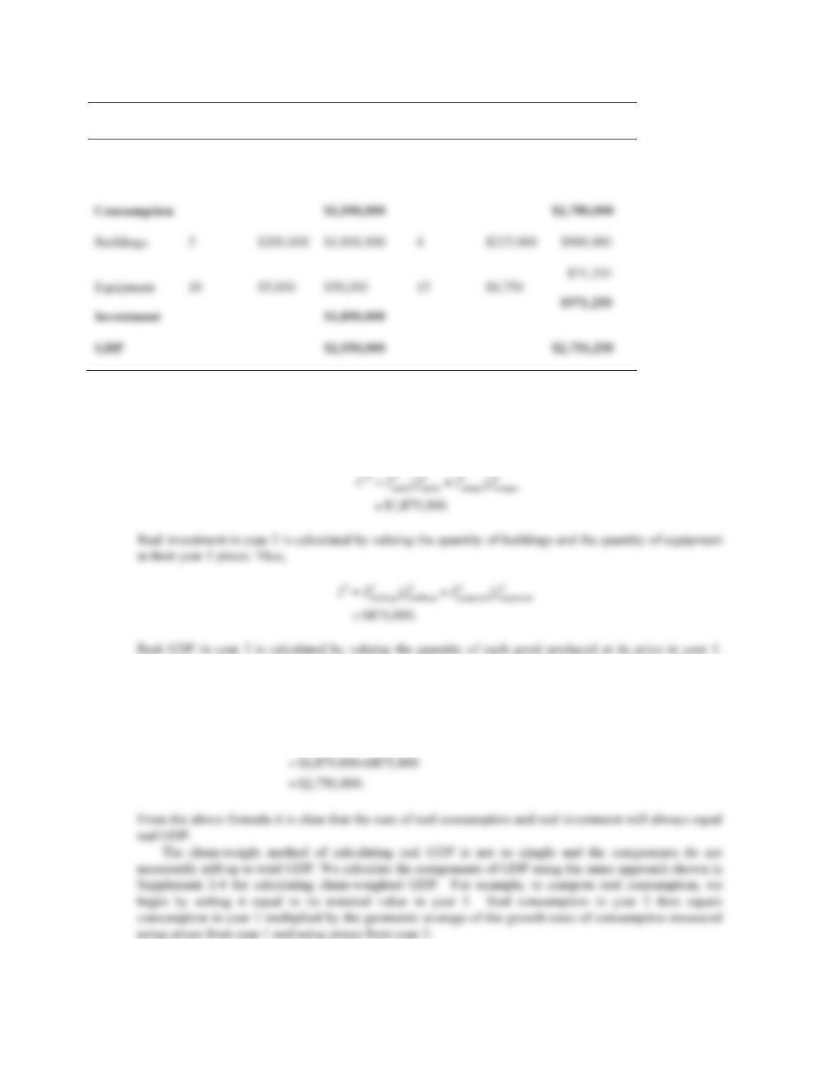
Table 3 Calculating GDP and Its Components
Quantity
Year 1
Price
Expenditures
Quantity
Year 2
Price
Expenditures
Apples
4,000,000
$.25
$1,000,000
3,500,000
$.28
$980,000
Oranges
1,000,000
$.5
$500,000
2,000,000
$.4
$800,000
Calculating real GDP under the fixed–weight method in this economy is easy. Suppose year 1 is the
base year. Then real consumption and investment are $1.5 million and $1.1 million, respectively, in year 1,
and real GDP is $2.6 million. In year 2, real consumption is calculated by valuing the quantity of apples
and the quantity of oranges at their year 1 prices. Thus,
Thus,
Real GDP2=P
apples
1Qapples
2+P
oranges
1Qoranges
2+P
buildings
1Qbuildings
2+P
equipment
1Qequipment
2
=C2+I2
$200,000
$1,000,000
$225,000
$900,000

Similarly, real investment in year 2 is equal to real investment in year 1 multiplied by the geometric
average of the growth rates of investment measured using prices from year 1 and using prices from year 2:
The formula used to calculate real GDP under the chain–weight method is not the sum of the formulas
used to calculate the components (as is the case under a fixed–weight calculation). Therefore, the
components do not sum to GDP. The formula for real GDP in year 2 is:
The residual is
apples
1Qapples
2+ P
oranges
1Qoranges
2
⎛
apples
2Qapples
2+ P
oranges
2Qoranges
2
⎛
=1.2099 ×$1,500,000
=$1,814,850.
GDP2−C2+I2
( )
=$2,676,990 −$1,814,850 +$872,340
( )
38
CASE STUDY EXTENSION
2-5 Defining National Income
A case study in Chapter 2 of the text describes the 2013 comprehensive revision of the National Income
2003. With that revision, the Bureau adopted the definition of national income recommended by the
System of National Accounts 1993 1, the principal international guidelines for national accounts data. 2
Since 1993, the Bureau gradually has adopted most of the major changes recommended by these
international guidelines, including the move in 1996 to chain–weight indexes for measuring changes in real
GDP and prices (see Supplement 2–4). As the Bureau noted in announcing its 2003 revision, “integration
of the world’s monetary, fiscal, and trade policies has led to a growing need for international
harmonization of economic statistics. Many of the definitional changes presented in this year’s revision
LECTURE SUPPLEMENT
2-6 Seasonal Adjustment and the Seasonal Cycle
Economists use various techniques to describe economic data. One set of techniques involves
decomposing data series into constituent subseries that can be added together to give the total series. As an
example, economists often separate GDP into a long–run, or trend, component and a short–run, or business
cycle, component.1 Another decomposition involves removing the seasonal component from economic
Robert Barsky and Jeffrey Miron decided instead to look at the seasonal component of the data.3
Interestingly, they found that the same sort of regularities that are observed in business cycle data also
show up in seasonal data. Moreover, they found that seasonal fluctuations are significant in the sense that
they account for much of the variation in detrended data. Seasonal fluctuations were found in all major
components of GDP.
All major components of GDP with the exception of fixed investment display the same seasonal
pattern: a large decline in the first quarter, small declines in the second and third quarters, and a large
increase in the fourth quarter. Fixed investment shows declines in the first and fourth quarters and
important for the business cycle as some theories suggest.4 Whereas seasonal and business cycles may be
initially generated by different shocks, they may be driven by similar propagation mechanisms.5
The finding that money is procyclical in seasonal data indicates that the causal relationship runs from
output to money, and not vice versa (since monetary expansions presumably do not cause Christmas). The
view that money may be endogenous at the cyclical level is important to real–business–cycle theory.
40
ADDITIONAL CASE STUDY
2-7 Measuring the Price of Light
According to William Nordhaus, unmeasured changes in quality dramatically overestimate the true rise in
the cost of living, as measured by the consumer price index (CPI).1Nordhaus uses a simple example of
estimating the price of light to illustrate the importance of quality changes and the effect that not
accounting for these changes can have on the measurement of inflation. Nordhaus traces the use of
artificial light from fire to fat burning lamps to candles to kerosene lamps to the electric light bulb.
tripled in the last 190 years, while consumer prices have risen tenfold. If, rather than measuring the price
of a good that produces light, one measures the price of a lumen hour of light, the results are very
different. This “true price” of light has declined precipitously since 1800. The nominal price of 1000
lumen hours of light has declined from $0.40 in 1800 to $0.03 in 1900 to nearly $0.001 in 1992, as shown
in Table 1. The real price has fallen even more, from $4.30 in 1800 to $0.43 in 1900 to nearly $0.001 in
1992. Comparing the real price of light as measured by the traditional and true price indexes, Nordhaus
states that the traditional price of light overestimates the true price by a factor of 900 over the period
1800–1992, or 3.6 percent per year.
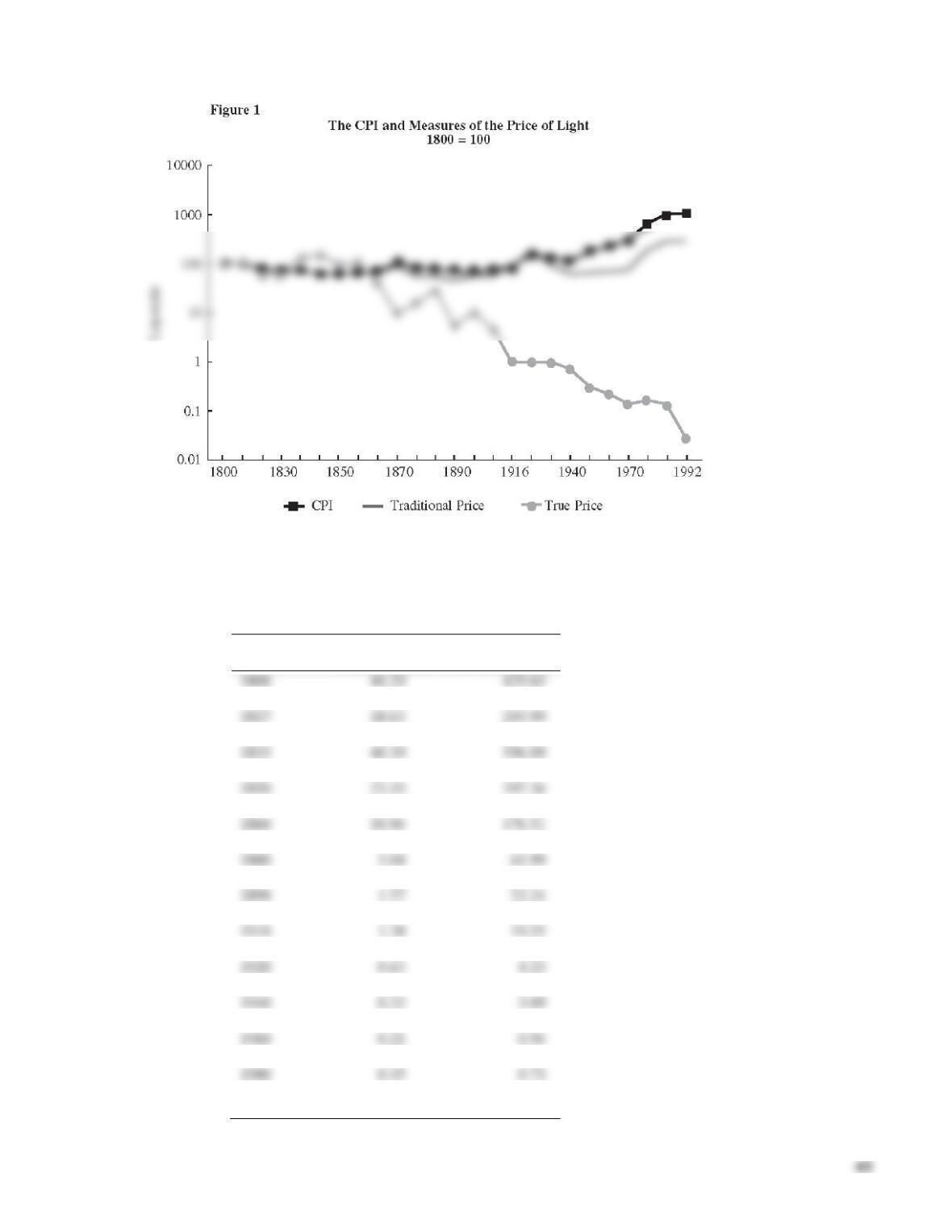
Table 1 True Price of Light (price per 1000 lumen hours)
Year
Current
Price (cents)
Real (1992)
Price (cents)
1800
40.29
429.63
1818
40.87
430.12
1827
18.63
249.99
1830
18.32
265.66
1835
40.39
596.09
1840
36.94
626.77
1850
23.20
397.36
1855
29.78
460.98
1860
10.96
176.51
1870
4.04
41.39
1880
5.04
1883
9.23
127.79
1890
1.57
23.24
1900
2.69
42.90
1910
19.55
1916
0.85
4.28
1920
0.63
4.23
1930
0.51
4.10
1940
0.32
3.09
1950
0.24
1.35
1960
0.21
0.94
1970
0.18
0.61
1980
0.45
0.73
1990
0.60
0.63
1992
0.12
0.12
42
LECTURE SUPPLEMENT
2-8 Improving the CPI
The Bureau of Labor Statistics (BLS) has made changes to the consumer price index in an effort to
measure inflation more accurately. Some of these changes address the measurement problems discussed in
Chapter 2 of the text and are part of an ongoing program at the BLS to improve the CPI.1 These changes
involve problems associated with substitution bias, introduction of new goods, and quality improvements.
Substitution Bias
Second, the BLS adopted a new policy of updating the market basket more frequently starting in
January 2002. The weights in the market basket are now updated on a two–year schedule, rather than the
roughly ten–year schedule of the past. Because of production lags in the collection of data, the weights for
the January 2010 update come from the average expenditure pattern of 2007–2008. These weights will be
updated again starting with the January 2012 index using the spending patterns from 2009–2010, and
New Goods
The BLS in 1999 incorporated improved procedures to update its sample of stores and items more rapidly,
helping ensure that new brands of products and new stores are included in the index more quickly than in
the past. Likewise, the shorter two–year time lag in updating the market basket itself will ensure that
completely new products are more rapidly introduced into the index. As the text points out, a greater
Consumer Price Index,” Monthly Labor Review, December 1996; and K.V. Dalton, J.S. Greenlees, and K.J. Stewart, “Incorporating a Geometric
Mean Formula into the CPI,” Monthly Labor Review, October 1998.
2 See M.J. Boskin, E.R. Dulberger, R.J. Gordon, Z. Grilliches, and D.W. Jorgenson, “Consumer Prices, the Consumer Price Index, and the Cost of
Living,” Journal of Economic Perspectives, 12(1), Winter 1998

Quality Improvements
The BLS has introduced quality adjustments to the prices of an expanding array of products over the years,
recently adding adjustments for apparel (1991), personal computers (1998), and televisions (1999). Some
economists believe that mismeasurement of improvements in quality is the single largest source of upward
bias in the CPI. But others point out that deterioration in quality may have occurred for some products.
The quality of air travel, for example, is generally thought to have declined in recent years as competition
44
ADDITIONAL CASE STUDY
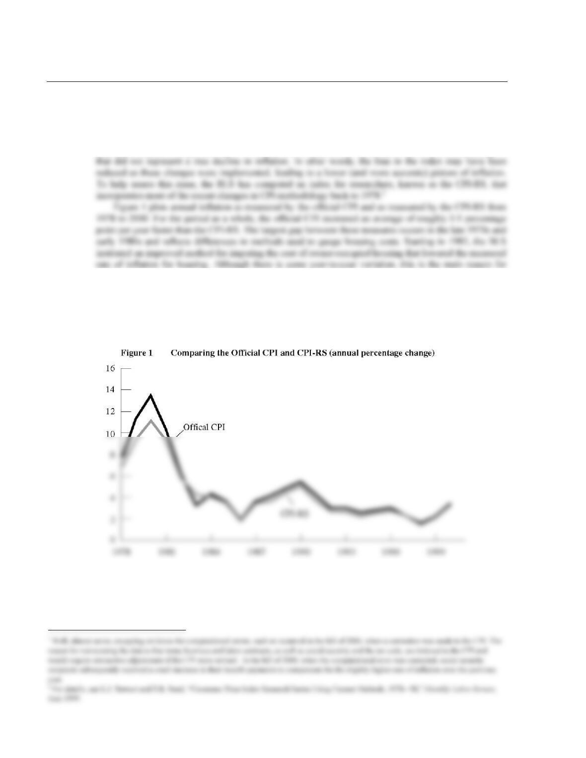
2-9 CPI Improvements and the Decline in Inflation During the 1990s
An important feature of the official CPI is that the series is never revised and so recent improvements in
the index are not introduced into the historical data.1 As a consequence, some of the decline in inflation
over the 1990s was probably due to methodological changes in the index—such as improvements in the
treatment of generic drugs starting in 1995 and various improvements in adjustments for quality change—
much of the gap between these series in the period before 1983. As new methods were introduced during
the 1990s, the gap continued to shrink. For 2000, the methodologies are the same and so there is no
difference between inflation as measured by the two indexes. For the 1990s, the CPI–RS rose about 0.25
percentage point per year less than the official CPI and thus can account for only about one–eighth of the
2-percentage–point decline in official CPI inflation between 1990 and 2000.
Source: U.S. Department of Labor, Bureau of Labor Statistics. Data are annual percentage change.
ADDITIONAL CASE STUDY
2-10 The Billion Prices Project
The CPI is based on thousands of prices for individual goods and services that are collected each month by
workers for the Bureau of Labor Statistics who visit retail stores. Two researchers recently proposed
another way to gather price data. MIT economists Alberto Cavallo and Roberto Rigobon use the Internet
to track prices charged by 300 online retailers for about five million items sold in 70 different countries.
They then use these data to compute overall price indices for the 70 countries.1
46
LECTURE SUPPLEMENT
2-11 Alternative Measures of Unemployment
The text defines unemployment as the percentage of the labor force unemployed at a particular time. The
labor force consists of individuals 16 and over who currently have a job (the employed) or do not have a
job but are actively seeking work (the unemployed). An individual who does not have a job and is not
looking for work is not considered part of the labor force.
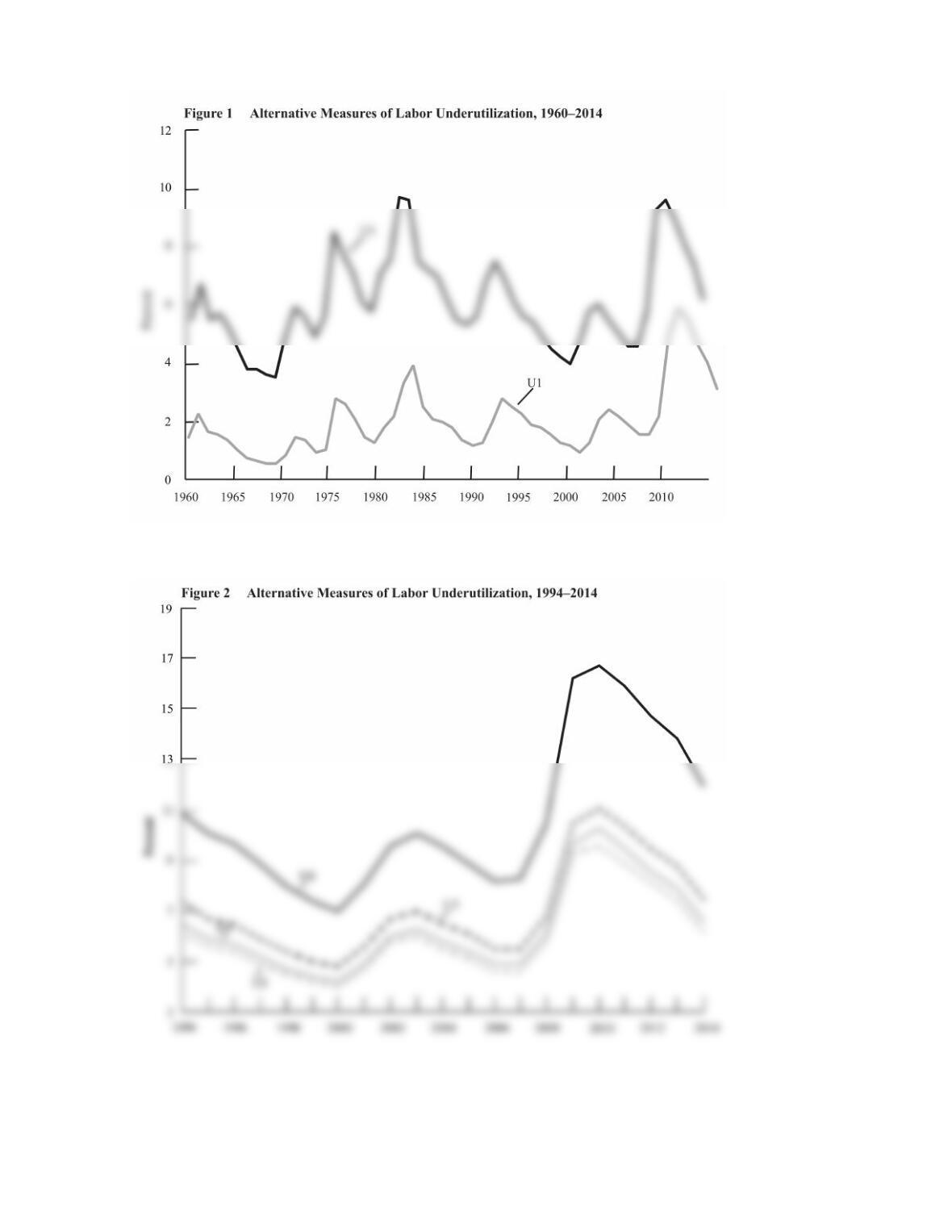
force plus all marginally attached workers.
U6: All unemployed persons plus all marginally attached workers, plus all persons employed part time
for economic reasons, as a percentage of the civilian labor force plus all marginally attached workers.
U3 is known as the official unemployment rate and corresponds to the definition of the unemployment rate
given in the text. U1 and U2 examine a subset of the unemployed as a percentage of the civilian labor
discouragement, transportation problems, and child–care problems. U4 and U5 thus measure the extent to
which the economy is not utilizing potential labor resources. U6 measures the extent to which both
potential (the marginally attached workers) and existing (part–time workers who would like to work full
time) labor resources are not utilized.
As shown in Figure 2, these three measures follow the cyclical pattern of the official unemployment
rate (U3), falling during the expansion of the 1990s and rising during the recessions of 2001 and 2007–
47
Source: U.S. Department of Labor, Bureau of Labor Statistics
Source: U.S. Department of Labor, Bureau of Labor Statistics.
ADDITIONAL CASE STUDY
2-12 Improving the National Accounts
Economists have long been aware that the statistics in the national accounts are imperfect. Some of these
imperfections simply have to do with the difficulties of precisely defining and/or measuring the variables
that economists care about. Some critics charge, however, that there are fundamental problems with the
system of national accounts. One set of arguments challenges the presumption that measures of income,
such as Gross Domestic Product, tell us anything useful about individuals’ welfare or overall well–being.
Another set of arguments holds that the national accounts are dangerously misleading because they fail to
take account of the depletion of natural resources and other environmental concerns.
This ambitious new measure thus focused on consumption. It added some components of government
expenditures, such as recreation outlays, to private consumption, but not others, such as national defense
(termed a “regrettable”). It reclassified some elements of private consumption (such as education and
health expenditures and consumption of durables) as investment and subtracted other components, such as
personal business expenses. Nordhaus and Tobin also added in an imputed value for leisure and other
nonmarket uses of time.
The two most important of the many adjustments Nordhaus and Tobin made were the exclusion of
regrettables (which they found to be an increasing fraction of GDP) and the imputations for leisure and
nonmarket work. The latter correction proved to be sensitive to different assumptions about the effects of