e. The government-purchases multiplier is 2.5. When Grises, the multiplier is
smaller than 1/(1 – MPC) because any increase in income will be accompanied by
an increase in taxes. Hence, the increase in disposable income in each round will
be smaller than the increase in income. Alternatively, the slope of the planned
expenditure curve becomes MPC(1 – t), where tequals the income tax rate. Hence,
the multiplier becomes 1/[1 – MPC(1 – t)].
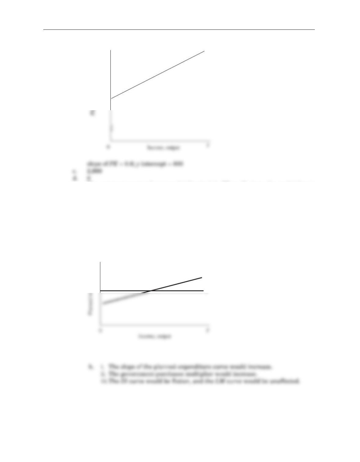
6. a. Planned investment might increase as Yrises (leading to the positively sloped line
below) if investment depends on profits or sales expectations (along with r) and
either or both of these rise along with Y.
212 Answers to Selected Student Guide Problems
PE PE
800
I‘
I
Data Questions
1. Table 10–7
(1) (2) (3) (4) (5) (6)
Nominal M2
in December % Change in GDP Deflator Real M2 % Change
Year ($ in billions) M2 (2000 = 100) M2/Pin M2/P
1979 1,473.7 49.5 2,977.2
8.6 –0.5
1980 1,599.8 54.0 2,962.6
The
LM
curve implies that changes in the real money supply are the appropriate
measures of monetary conditions. Using this measure, the Fed pursued mildly
contractionary monetary policy between 1979 and 1980, neutral policy between
Problems
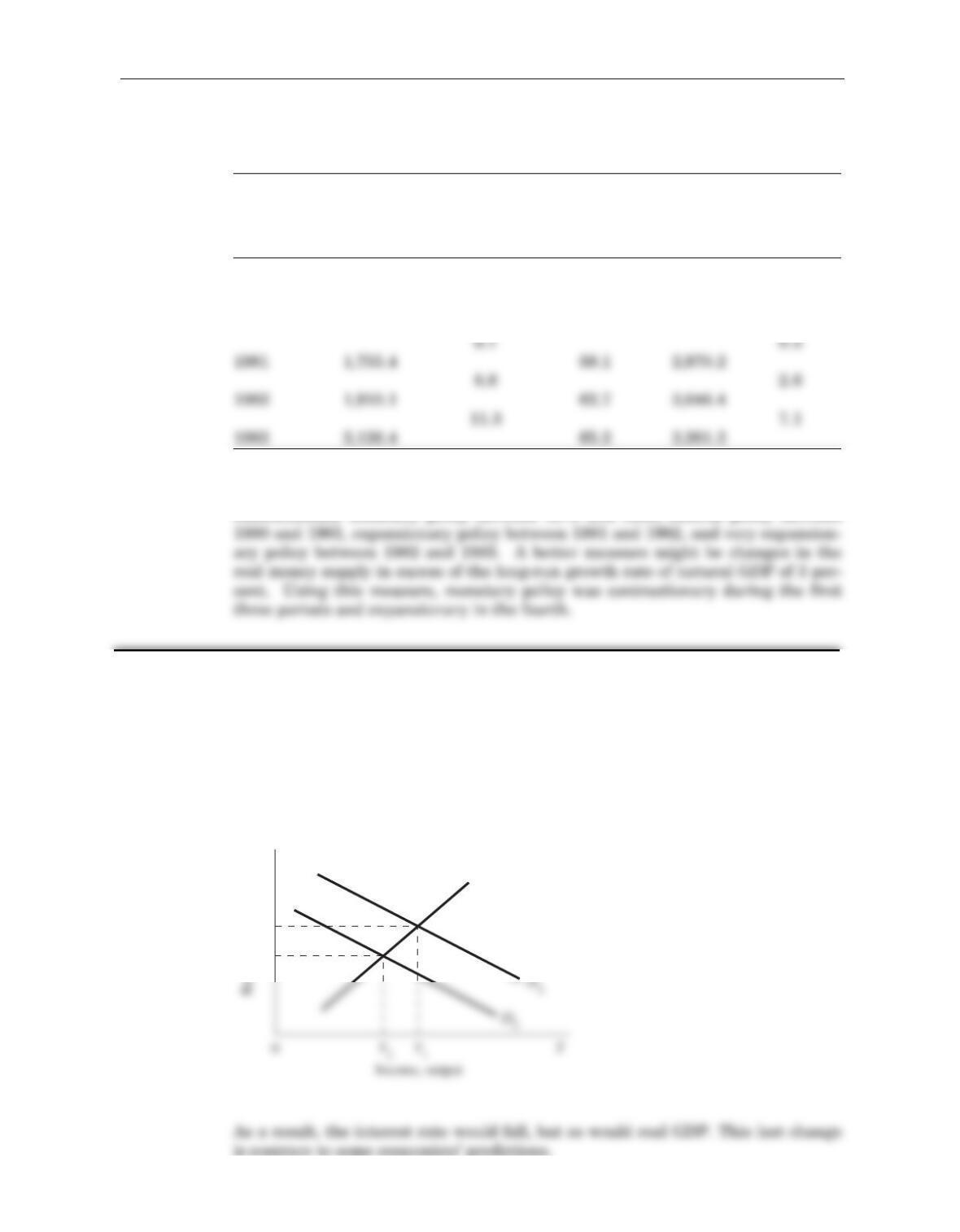
4. a. The deficit would fall. The IS curve would shift to the left.
Graph for Problem 4(a)
Chapter 10 Aggregate Demand I 213
CHAPTER 11 Aggregate Demand II
r
r1
r2
LM

b. If expansionary monetary policy is pursued simultaneously, the interest rate and
the deficit will still fall and real income may actually rise.
Graph for Problem 4(b)
13. a. Graph for Problem 13(a)
14. If the money supply M increased as the interest rate increased, the money supply
curve would be upward sloping.
214 Answers to Selected Student Guide Problems
r
LM1
LM2
r1
A
r
r2
LM1(πe = 0)
LM2(πe = –10)
r1 + 10
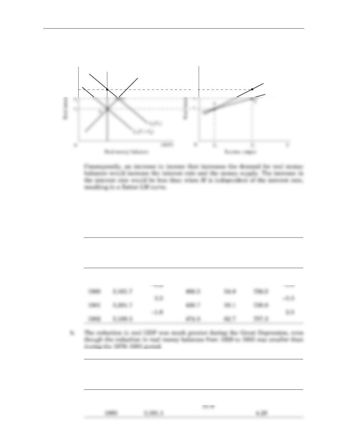
Graph for Problem 14
Data Questions
1. a. Table 11–1
(1) (2) (3) (4) (5) (6) (7)
Real GDP % M1 GDP %
in billions of Change in in Dec. Deflator Real M1 Change in
Year 2000 dollars Real GDP ($ in billions) (2000 = 100) (= M1/P) Real M1
1979 5,173.4 381.8 49.5 771.3
2. a. Table 11–2
(1) (2) (3) (4)
Real GDP % Interest Rate
in billions of Change in on 10-Year U.S.
Year 2000 dollars Real GDP Treasury Securities
1960 2,501.8 4.12
Chapter 11 Aggregate Demand II 215
B
B
LM
M/P
r
r2
‹
(M/P)
‹
LM
‹
r
r2
‹
b. Since the interest rate remained relatively constant while real GDP rose, it may
be presumed that both the
LM
and the
IS
curves shifted to the right and that the
horizontal shift was the same for both curves. Consequently, the Federal Reserve
must have increased the money supply during this period.
Data Questions
1. a. and b.
Table 13–1
(1) (2) (3) (4) (5) (6)
Real GDP Actual Predicted
(billions % Civilian Change in Change in
of 2000 Change in Unemployment Unemployment Unemployment
Year dollars) Real GDP Rate (%) Rate Rate
2001 9,890.7 4.7
Problems
6. a. If capital gains taxes are reduced, the after-tax return to saving would increase.
This might increase total saving, which would spur additional investment in a
closed economy or a large open economy.
b. A capital gains tax reduction on past acquisitions will increase the after-tax
216 Answers to Selected Student Guide Problems
CHAPTER 13 Aggregate Supply and the Short-Run
Tradeoff Between Inflation and
Unemployment
CHAPTER 15 Stabilization Policy
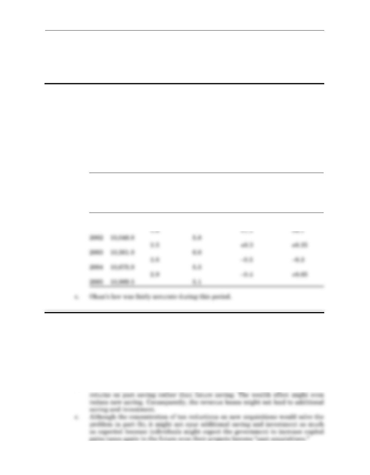
Data Questions
1. a.
Table 15–1
(1) (2) (3) (4) (5)
Real Actual
GDP Real GDP Unemployment Actual
Growth Growth Rate Unemployment
Year Forecast (%) Rate (%) Forecast (%) Rate (%)
Problems
4. According to the traditional view, the future reduction in government spending would
have no effect on the sum of current and expected future income, current consumption,
or current private saving. According to the Ricardian view, a future reduction in gov-
ernment purchases will be accompanied by an expected future reduction in taxes. This
Data Questions
1. a. Table 16–3
(Data in billions of $)
(1) (2) (3) (4) (5)
Total Federal Total Federal Official Gross Federal
Fiscal Government Government Federal Budget Debt Held by
Year Receipts Outlays Surplus Public (end of year)
2003 1,782.5 2,160.1 –377.6 3,913.4
Chapter 16 Government Debt 217
CHAPTER 16 Government Debt
b. Table 16–4
(1) (2) (3) (4) (5)
Price Gross Federal Debt Approximate
Deflator for Held by Public (end “True” Federal
Calendar GDP Percentage of
preceding
fiscal year) Budget Surplus
Year (2000 = 100) Change ($ in billions) ($ in billions)
2004 109.5 3,913.4 –287.5
Problems
4. a. C1= 100; C2= 125; S= 20
b. C1= 93.33; C2= 140; S= 26.67
6. a. A country with a rapidly increasing population will have a higher saving rate (and
a lower aggregate APC) than a country with a steady population because each suc-
cessive generation of workers, who do the saving, will be larger than the preceding
10. After the legislation was passed, all the future tax cuts became expected. According to
this theory, people’s permanent incomes rose (and, hence, their consumption rose) only
in the first year, 1981, which would be the only year in which consumption changed as
a result of the tax changes unless people had borrowing constraints.
Data Questions
1. a. Table 17–5
(1) (2) (3) (4)
Real Real
Consumption Disposable Average
Expenditures Income Propensity to
Year ($ in billions) ($ in billions) Consume (APC)
218 Answers to Selected Student Guide Problems
CHAPTER 17 Consumption

b. Percentage change in real disposable income equals 249.1 percent; percentage
change in APC is 8.2 percent.
2. a. Table 17–6
(1) (2) (3) (4)
Consumption Disposable Average
Expenditures Income Propensity to
Year ($ in billions) ($ in billions) Consume (APC)
1967 507.8 575.3 0.883
Problems
9. a. An investment tax credit of 8 percent allows firms to deduct 8 percent of their
investment expenditures from their taxes.
b. The cost of capital declines at each real interest rate. Consequently, the IS curve
shifts to the right. The LM curve does not shift.
Chapter 18 Investment 219
CHAPTER 18 Investment
Data Questions
1. a. Table 18–3
(1) (2) (3) (4) (5)
Real
Real Nonresidential Real
Nonresidential Investment in Real Change in
Investment in Equipment Residential Business
Year Structures and Software Investment Inventories
($ in billions) ($ in billions) ($ in billions) ($ in billions)
1998 294.5 745.6 418.3 72.6
2. Some of the data were not yet available when this book went to press.
Table 18–14
(1) (2) (3) (4) (5) (6)
Average Percentage Real Percentage
Value of Change GDP Change
S&P in S&P Quarter (Billions of in Real
Month 500 Index 500 Index and Year 2000 $) GDP
August 2008 1,281.47 2008: Q4 11,522.1
–31.9 –1.6
November 2008 873.28 2009: Q1 11,340.9
________ ________
February 2008 ________ 2009: Q2 ________
220 Answers to Selected Student Guide Problems

Problems
Data Questions
1. a. and b.
Table 19–2
(1) (2) (3) (4) (5) (6)
Monetary Base M1M2
in Dec. in Dec. M1 Money in Dec. M2 Money
Year ($ in billions) ($ in billions) Multiplier ($ in billions) Multiplier
1987 239.8 750.2 3.13 2,831.3 11.81
c. If the Fed had preset targets for
M
1, it would have had to continually increase its
target for the monetary base after 1987 to offset the decline in the
M
1 money mul-
tiplier. If the Fed had preset targets for
M
2, it would have had to increase its tar-
get for the monetary base between 1987 and 1997 to offset the decrease in the
M
2
Chapter 19 Money Supply and Money Demand 221
CHAPTER 19 Money Supply, Money Demand,
and the Banking System
