CHAPTER 2
Measurement
KEY IDEAS IN THIS CHAPTER
1. Measurements of key macroeconomic variables such as gross domestic product
2. GDP can be measured using the product approach, the expenditure approach, or the
3. There are two approaches to measuring real GDP: choosing a base year and chain-
4. Three key labour market variables are the unemployment rate, the participation rate,
NEW IN THE FOURTH EDITION
2. All data and graphs have been updated.
TEACHING GOALS
Students must understand the importance of measuring aggregate economic activity.
Macroeconomics hopes to produce theories that provide useful insights and policy
conclusions. To be credible, such theories must produce hypotheses which evidence
could possibly refute. Macroeconomic measurement provides such evidence. Without
macroeconomic measurements, macroeconomics could not be a social science, and would
rather consist of philosophizing and pontificating. Market transactions provide the most
simple and direct measurements. Macroeconomists’ most basic measurement is Gross
Domestic Product (GDP), the value of all final goods and services produced in an
economy during a given period of time.
Instructor’s Manual for Macroeconomics, Fourth Canadian Edition
In Canada, Statistics Canada’s National Income and Expenditure Accounts provide the
official estimates of GDP. These accounts employ their own set of accounting rules to
ensure internal consistency and to provide several separate estimates of GDP. These
separate estimates are provided by the product accounts, the expenditure accounts, and
the income accounts. The various accounting conventions may, at first glance, be rather
dry and complicated. However, students can only easily digest the material in later
chapters if they have a good grounding in the fundamentals.
GDP changes through time because different amounts of goods and services are
produced, and such goods and services are sold at different prices. Standards of living are
determined by the amounts of goods and services produced, not by the prices they
command in the market. While GDP is relatively easy to measure, the decomposition of
CLASSROOM DISCUSSION TOPICS
As the author demonstrates in the textbook, much of this material is best learned by
example. Rather than simply working through the examples from the text or making up
your own, the material may resonate better if students come up with their own examples.
They can start by picking a single good, and by the choice of their numbers, provide their
own implied decomposition of output into wage and profit income. Later on, encourage
them to suggest intermediate input production, inventory adjustments, international
transactions, and a government sector. Such an exercise may help assure students that the
identities presented in the text are more than simply abstract constructions.
Canada Pension Plan benefits are indexed to the Consumer Price Index. Explain with an
example exactly how these adjustments are made. Ask the students if they think that this
procedure is “fair.” Another topic for concern is the stagnation in the growth of measured
real wages. Real wages are measured by dividing (for example) average hourly wages
paid in manufacturing by the consumer price index. Ask students if measured changes in
Chapter 2: Measurement
productive activities done in and around the house by members of the household. Point
out to students that in Canada (as well as in many other industrialized countries) many
children receive day care from commercial providers. In many countries in Asia and
Africa, this is unknown; children are almost all cared for by relatives. Then ask: how
would this affect comparisons of GDP per capita? Would this difference have any
implication for welfare levels?
The text discusses why unemployment may or may not be a good measure of labour
market tightness. Another interpretation of the unemployment rate is that it has an inverse
OUTLINE
1. Measuring GDP: The National Income and Expenditure Accounts
a) What Is GDP and How Do We Measure It?
i) GDP: Value of Final Output Produced Domestically
ii) Statistics Canada’s National Income and Expenditure Accounts
b) The Product Approach to Measuring GDP
i) Value Added
ii) Intermediate Goods Inputs
c) The Expenditure Approach
i) Consumption
ii) Investment
iii) Government Expenditures
iv) Net Exports
d) The Income Approach
i) Wage Income
ii) After-Tax Profits
iii) Interest Income
iv) Taxes
v) The Income–Expenditure Identity
e) An Example with Inventory Investment
f) An Example with International Trade
g) Gross National Product (GNP)
i) Treatment of Foreign Income
ii) GNP = GDP + Net Foreign Factor Payments from Abroad
h) What Does GDP Leave Out?
i) GDP and Economic Welfare
(1) Income Distribution
(2) Non-Market Activity
Instructor’s Manual for Macroeconomics, Fourth Canadian Edition
ii) Measuring Market Activity
(2) Valuing Government Expenditures
i) The Components of Aggregate Expenditure
i) Consumption
(1) Durable Goods
(3) Non-Durable Goods
(4) Services
ii) Investment
(1) Fixed Investment: Nonresidential and Residential
(2) Inventory Investment
iii) Net Exports
iv) Government Expenditures
(1) Government Consumption
(3) Treatment of Transfer Payments
2. Nominal and Real GDP and Price Indices
a) Impact of Price Changes
i) Price Index versus Inflation Rate
ii) Real and Nominal Changes
b) Real GDP
i) Output Valued at Base Year Prices
ii) Chain-Weighted Real GDP
c) Measures of the Price Level
i) Implicit GDP Price Deflator
3. Savings, Wealth, and Capital
a) Stocks and Flows
b) Private Disposable Income and Private Sector Saving
i) TINTTRNFPYY d−+++=
c) Government Surpluses, Deficits, and Government Saving
i) GINTTRTS g−−−=
d) National Saving:
Chapter 2: Measurement
e) Saving, Investment, and the Current Account
i) NFPNXIS ++=
ii) CAISNFPNXCA +=+=
f) The Stock of Capital
4. Labour Market Measurement
a) Statistics Canada’s Categories
i) Employed
ii) Unemployed
iii) Not in the Labour Force
b) The Unemployment Rate
Number unemployed
Unemployment Rate Labor force
=
c) The Participation Rate
TEXTBOOK QUESTION SOLUTIONS
Problems
1. Product accounting adds up value added by all producers. The wheat producer has no
intermediate inputs and produces 3 million tonnes at $30/tonne for $90 million. The
bread producer produces 100 million loaves at $3.50/loaf for $350 million. The bread
producer uses $75 million worth of wheat as an input. Therefore, the bread producer’s
value added is $275 million. Total GDP is, therefore, $90 million + $275 million
= $365 million.
2. Coal producer, steel producer, and consumers.
a) i) Product approach: Coal producer produces 15 million tonnes of coal at
$5/tonne, which adds $75 million to GDP. The steel producer produces
$10 million tonnes of steel at $20/tonne, which is worth $200 million. The
steel producer pays $125 million for 25 million tonnes of coal at $5/tonne.
The steel producer’s value added is, therefore, $75 million. GDP is equal to
$75 million + $75 million = $150 million.
ii) Expenditure approach: Consumers buy 8 million tonnes of steel at $20/tonne,
iii) Income approach: The coal producer pays $50 million in wages and the steel
producer pays $40 million in wages, so total wages in the economy equal $90
million. The coal producer receives $75 million in revenue for selling 15
million tonnes at $5/tonne. The coal producer pays $50 million in wages, so
the coal producer’s profits are $25 million. The steel producer receives $200
b) There are no net factor payments from abroad in this example. Therefore, the
current account surplus is equal to net exports, which is equal to (−$10 million).
c) As originally formulated, GNP is equal to GDP, which is equal to $150 million.
3. Wheat and Bread
a) Following the product approach, value added by firm A is total revenue from
wheat sales (note that the inventory accumulation is treated as if the firm sold the
Chapter 2: Measurement
b) For the expenditure approach, consumption expenditure on bread, C = $100 000
+ $15 000 = $115 000 (note that imports of bread are included), investment in
c) For the income approach, in this case GDP is the sum of profits and wage income.
Profits for firm A are $150 000 – $50 000 = $100 000 (revenue minus wage costs,
4. Price and quantity data are given as the following:
Year 1
Good Quantity Price
Computers 20 $1000
Bread 10 000 $1.00
Year 2
Good Quantity Price
Computers 25 $1500
Bread 12 000 $1.10
a) Year 1 nominal GDP = 20 × $1000 + 10 000 × $1.00 = $30 000.
b) With year 1 as the base year, we need to value both years’ production at year 1
prices. In the base year, year 1, real GDP equals nominal GDP equals $30 000.
We next calculate chain-weighted real GDP. At year 1 prices, the ratio of year 2
real GDP to year 1 real GDP equals 1
g = ($37 000/$30 000) = 1.2333. We must
Instructor’s Manual for Macroeconomics, Fourth Canadian Edition
to 12 1.23496
c
ggg== .The percentage change chain-weighted real GDP from year
1 to year 2 is therefore approximately 23.5%.
c) To calculate the implicit GDP deflator, we divide nominal GDP by real GDP, and
then multiply by 100 to express GDP deflator as an index number. With year 1 as
the base year, base year nominal GDP equals base year real GDP, so the base year
d) Let us consider the possibility that year 2 computers are twice as productive as
year 1 computers. As one possibility, let us define a “computer” as a year 1
computer. In this case, the 25 computers produced in year 2 are the equivalent of
50 year 1 computers. Each year 1 computer now sells for $750 in year 2. We now
revise the original data as:
Year 1
Good Quantity Price
Year 1 Computers 20 $1000
Bread 10 000 $1.00
Year 2
Good Quantity Price
Year 1 Computers 50 $750
Bread 12 000 $1.10
Chapter 2: Measurement
First, note that the change in the definition of a “computer” does not affect the
calculations of nominal GDP. We next compute real GDP with year 1 as the
base year. Year 2 real GDP, in year 1 prices is now 50 × $1000 + 12 000 × $1.00
5. Price and quantity data are given as the following:
Year 1
Good Quantity
(million kgs.)
Price
(per kgs.)
Broccoli 1500 $0.50
Cauliflower 300 $0.80
Year 2
Good Quantity
(million kgs.)
Price
(per kgs.)
Broccoli 2400 $0.60
Cauliflower 350 $0.85
Instructor’s Manual for Macroeconomics, Fourth Canadian Edition
a) Year 1 nominal GDP = Year 1 real GDP
= 1500m. × $0.50 + 300m. × $0.80 = $990m.
b) Year 1 production (market basket) at year 1 prices equals year 1 nominal
GDP = $990m. The value of the market basket at year 2 prices is equal to
$900 + $255 = $1155.
6. If some goods are subject to price controls and these price controls are binding, then
current GDP will tend to be biased downward: the official price of a good subject to
price controls is less than the price which measures the true value of the good. As
7. What we know is that the quantity of Canadian currency outstanding is about $1670.
A safe assumption is that essentially all of this currency is held by residents of
Canada. What we need is an estimate of the average quantity of currency that the
average Canadian holds for use in market (non-underground) transactions. Suppose
that this quantity is $100. That leaves about $1400 per person that is being held for
8. Corn producer, consumers, and government.
a) i) Product approach: There are no intermediate goods inputs. The corn producer
grows 3 million tonnes of corn. Each tonne of corn is worth $50. Therefore,
GDP equals $150 million.
ii) Expenditure approach: Consumers buy 2 million tonnes of corn, so
consumption equals $100 million. The corn producer adds 0.5 million tonnes
iii) Income approach: Wage income is $60 million, paid by the corn producer. The
b) Private disposable income equals GDP ($150 million) plus net factor payments
(0) plus government transfers ($5 million in Canada Pension Plan benefits) plus
interest on the government debt ($10 million) minus total taxes
($30 million), which equals $135 million. Private saving equals private disposable
9. “Questionable financial activity” is essentially theft. If someone steals, there is no
contribution to GDP as something is simply transferred from one individual to
another. Possibly worse, the time and effort of the thief is pure waste for society, as
10. The dollar value of a transaction need not all be a contribution to GDP. Indeed,
typically only a fraction of any given transaction in the economy actually represents
something we should add to GDP. For example, the production of a given good could
11. The answers to parts (a) and (b) are in the table.
Year Capital when initial capital = 80 Capital when initial capital = 100
0 80 100
2 83.8 100
4 86.9 100
6 89.4 100
8 91.4 100
10 93.0 100
In the first case, where the initial quantity of capital was 80, with a constant quantity of
investment each period, the quantity of capital increases over time, but at a decreasing
rate (note the increment to the capital stock gets smaller each period). This happens
because, as the capital stock grows, the total amount of capital that depreciates each
period increases. The quantity of capital appears to be converging to some quantity, but
what is this quantity? When the quantity of capital is initially 100, then the capital stock
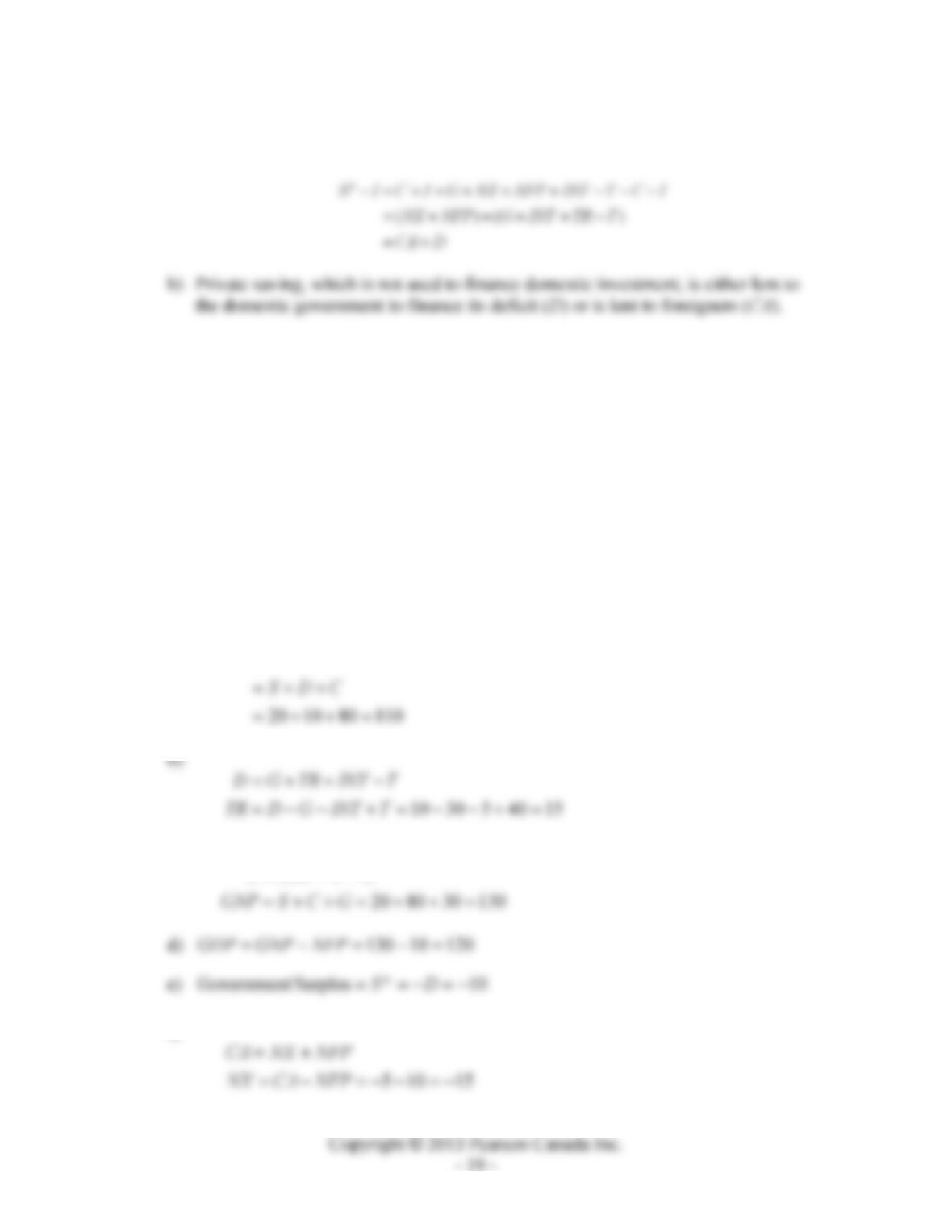
12. DCAIS p+=−
a) By definition:
pd
S Y C Y NFP TR INT T C=−=+ ++ −−
Chapter 2: Measurement
Next, recall that NXGICY +++= . Substitute into the equation above and
subtract I to obtain:
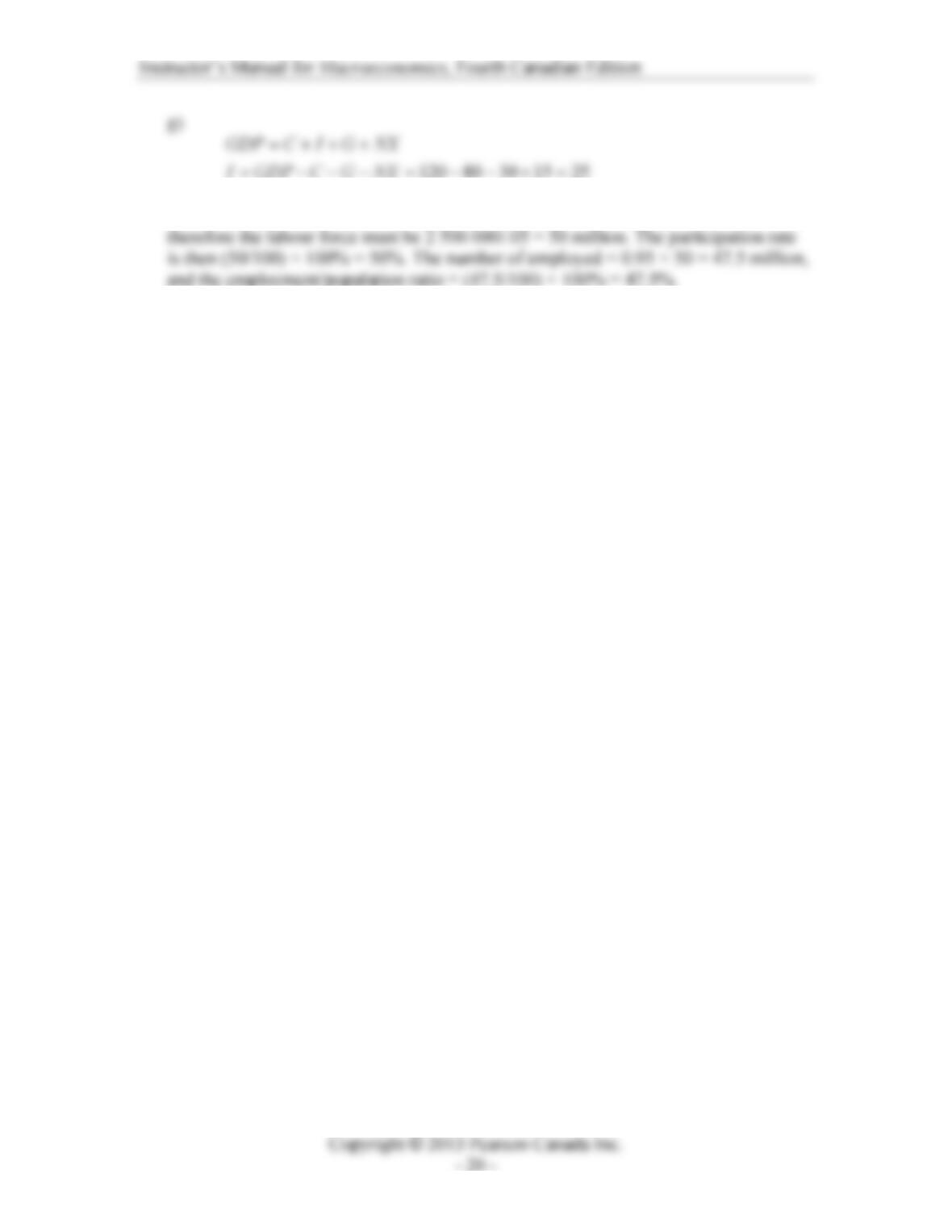
13. Assume the following:
20
5
10
80
30
40
5
10
=
−=
=
=
=
=
=
=
S
CA
NFP
C
G
T
INT
D
a)
+=
CSY pd
c)
−−=
GCGNPS
f)
14. If the unemployment rate is 5% and the number of unemployed is 2.5 million,