Chapter 2
Tools of Analysis for International
Trade Models
This chapter develops the theory underlying two dimensional general equilibrium trade models. In
particular, it considers topics such as the importance of relative (vs. nominal) prices in economic decision
The obvious intent of this chapter is to lay a theoretical foundation for the material that is to come. That is
why we discuss these topics in terms of a progression of assumptions. With the possible exceptions of our
increased emphasis on relative prices and our treatment of community indifference curves, most of this
material should be a review for the students. Nonetheless, it is a vital review—and we think it should
be emphasized as such—since virtually all of the tools of analysis used in later chapters are developed
here. Consequently, in teaching this material we try to emphasize to the students that despite all of the
discussion of autarky, we are building a model of international trade. However, these assumptions must
be made first.
◼ Chapter Outline
Introduction
Some Methodological Preliminaries
The Basic Model: Assumptions
Global Insights 2.1: World Response to Higher Relative Price of Oil
The Basic Model: Solutions
Measuring National Welfare
National Supply and Demand
Summary
Exercises
Appendix 2.1: Derivation of National Supply and Demand Curves
6 Husted/Melvin • International Economics, Ninth Edition
◼ Suggested Answers for the End-of–Chapter Exercises
1. Suppose that the economy produces three goods—raisins (R), soybeans (S), and textiles (T). What
would its PPF look like under conditions of constant opportunity costs? What would it look like with
increasing opportunity costs?
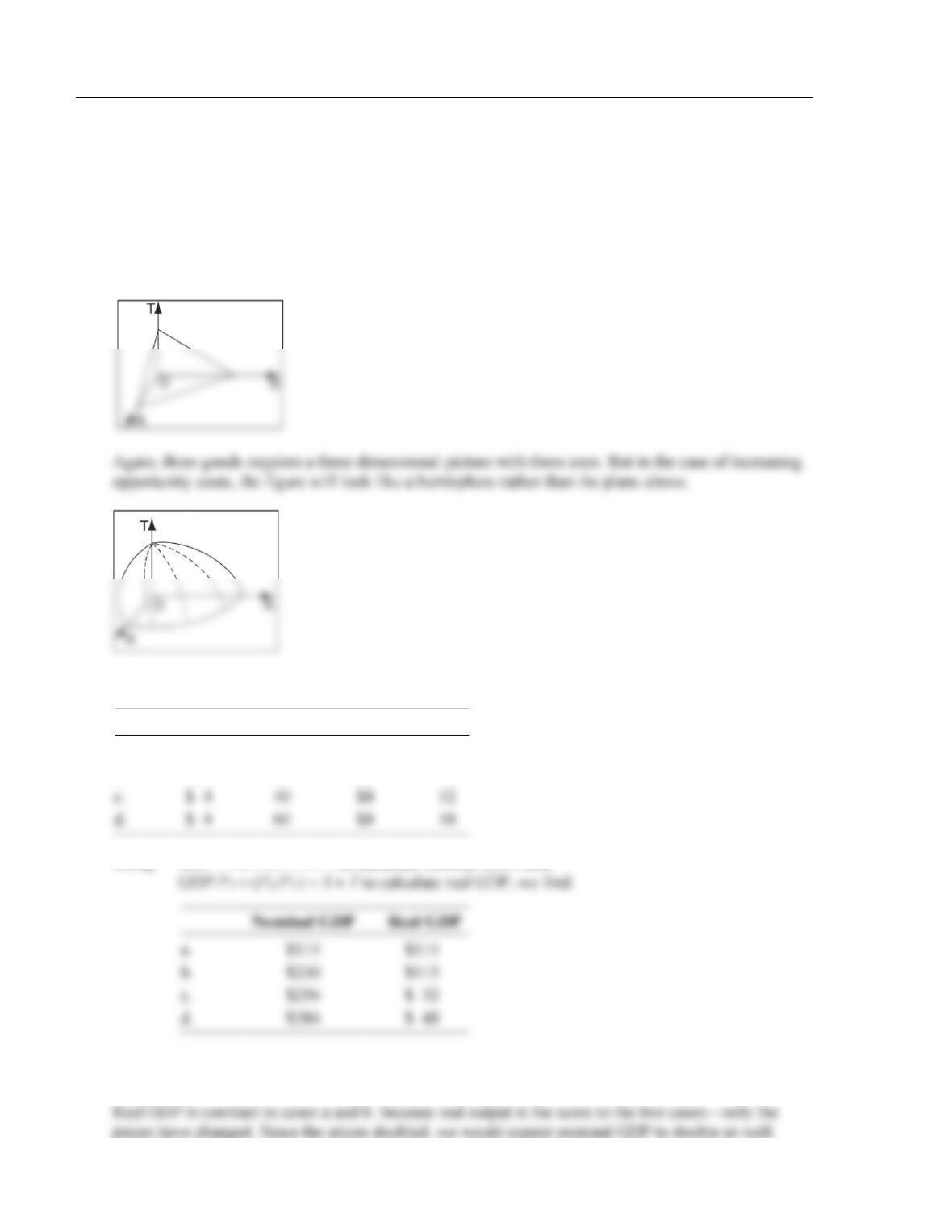
With three goods, we have a three dimensional figure with three axes, R, S and T. With constant
opportunity costs, the PPF is a plane instead of a line.
2. Using the following data, calculate the country’s nominal and real GDP levels.
PS
S
PT
T
a.
$ 5
20
$1
15
b.
$10
20
$2
15
c.
$ 4
40
$8
12
a.
b.
Using GDP = PS S + PT T to calculate nominal GDP, and
3. Using your calculations from Exercise 2, compare changes in nominal and real GDP between
cases a and b. Explain your result.
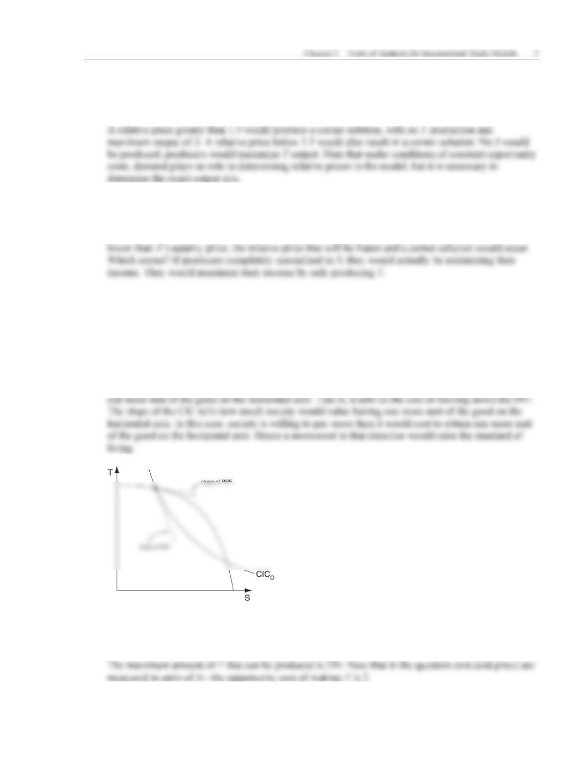
4. Suppose the economy is characterized by constant opportunity costs so that PS/PT = 1.5. Derive the
economy’s national supply schedule. How does it differ from the one derived in Figure A2.1 on
page 51? Explain.
5. Suppose that in world markets the relative price of S is lower than A’s autarky price. Would A be
a net exporter or importer of S? What would be the case for good T in country A in this situation?
This is exactly the situation discussed in the previous question. If the world’s relative price of S is
6. Derive country A’s national supply and demand curves for good T. Be careful how you label the axes!
Follow the example in text Figure 2.8.
7. If a country is at a point on its PPF where the slope of the PPF is flatter than the slope of the CIC
touching that same point, then the standard of living would rise if outputs of the two goods would
change so as to move down the PPF. True or false? Demonstrate and explain.
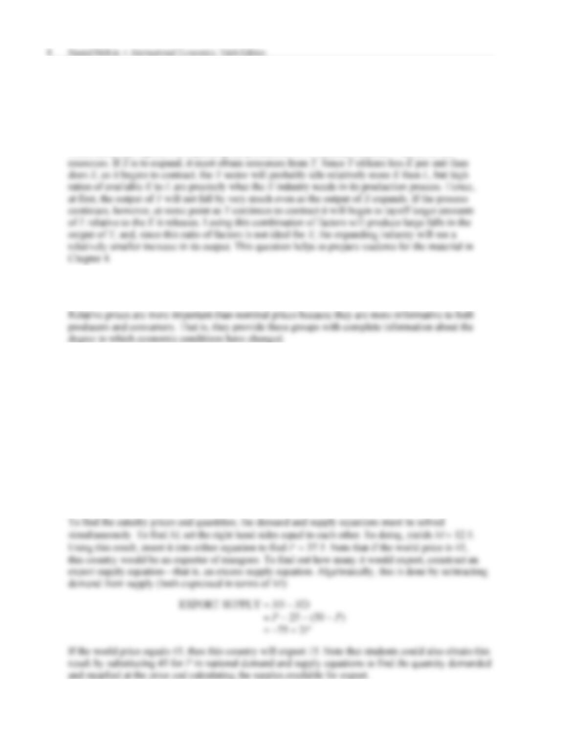
This statement is true. See the following graph. The slope of the PPF tells us the cost of producing
8. Suppose that country A produces two goods under conditions of constant opportunity costs. Given
its resources, the maximum S that it can make is 500 units and the opportunity cost of making T is 2.
What is the maximum amount of T that it can produce? Draw a graph and explain.
9. Suppose that a country produces two goods, X and Y, with two factors of production, K and L. The
production of good X always requires more K per unit than does the production of good Y. What does
this imply for the shape of the country’s PPF? Explain carefully.
In this case, the PPF will be concave to the origin, that is, it will be bowed out. Why? Suppose that
you start from a point of complete specialization in the production of Y (say, on the vertical axis).
Think about the logistics of expanding the production of X. Initially, industry Y has all of the
10. Why are relative prices more important for decisions about consumption and production than nominal
prices? Provide an example to illustrate your answer.
11. Suppose that a small, tropical country produces mangoes for domestic consumption and possibly for
export. The national demand and supply curves for mangoes in this country are given by the
following:
P = 50 − M (national demand)
P = 25 + M (national supply)
where P denotes the relative price of mangoes and M denotes the quantity of mangoes (in metric
tons).
a. Illustrate these relationships geometrically.
b. What is the autarky price and quantity exchanged?
c. Suppose that the world price of mangoes is 45. Will this small country export mangoes? If so,
how many tons?