Basic Econometrics, Gujarati and Porter
CHAPTER 2:
TWO-VARIABLE REGRESSION ANALYSIS: SOME BASIC IDEAS
2.2 The distinction between the sample regression function and the
population regression function is important, for the former is
2.3 A regression model can never be a completely accurate
description of reality. Therefore, there is bound to be some difference
2.4 Although we can certainly use the mean value, standard deviation
and other summary measures to describe the behavior the of the
2.7 (a) Taking the natural log, we find that ln Y
i
=
β
1
+
β
2
X
i
+ u
i
, which
2.8 A model that can be made linear in the parameters is called an
2.9 (a) Transforming the model as (1/Y
i
) =
β
1
+
β
2
X
i
makes it a linear
2.10 This scattergram shows that more export-oriented countries on
average have more growth in real wages than less export oriented
2.11 According to the well-known Heckscher-Ohlin model of trade,
countries tend to export goods whose production makes intensive
2.12 This figure shows that the higher is the minimum wage, the lower
is per head GNP, thus suggesting that minimum wage laws may
2.13 It is a sample regression line because it is based on a sample
of 15 years of observations. The scatter points around the regression
8
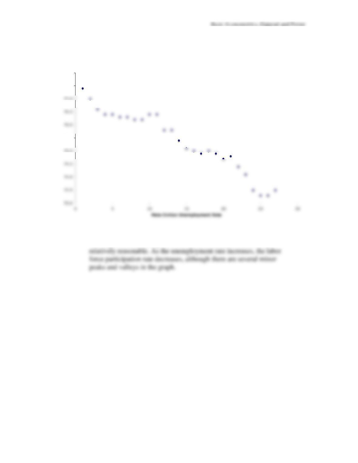
2.14 (a) The scattergram is as follows:
The negative relationship between the two variables seems seems
Male Labor Participation vs Unemployment
75.5
77.5
78.0
Basic Econometrics, Gujarati and Porter
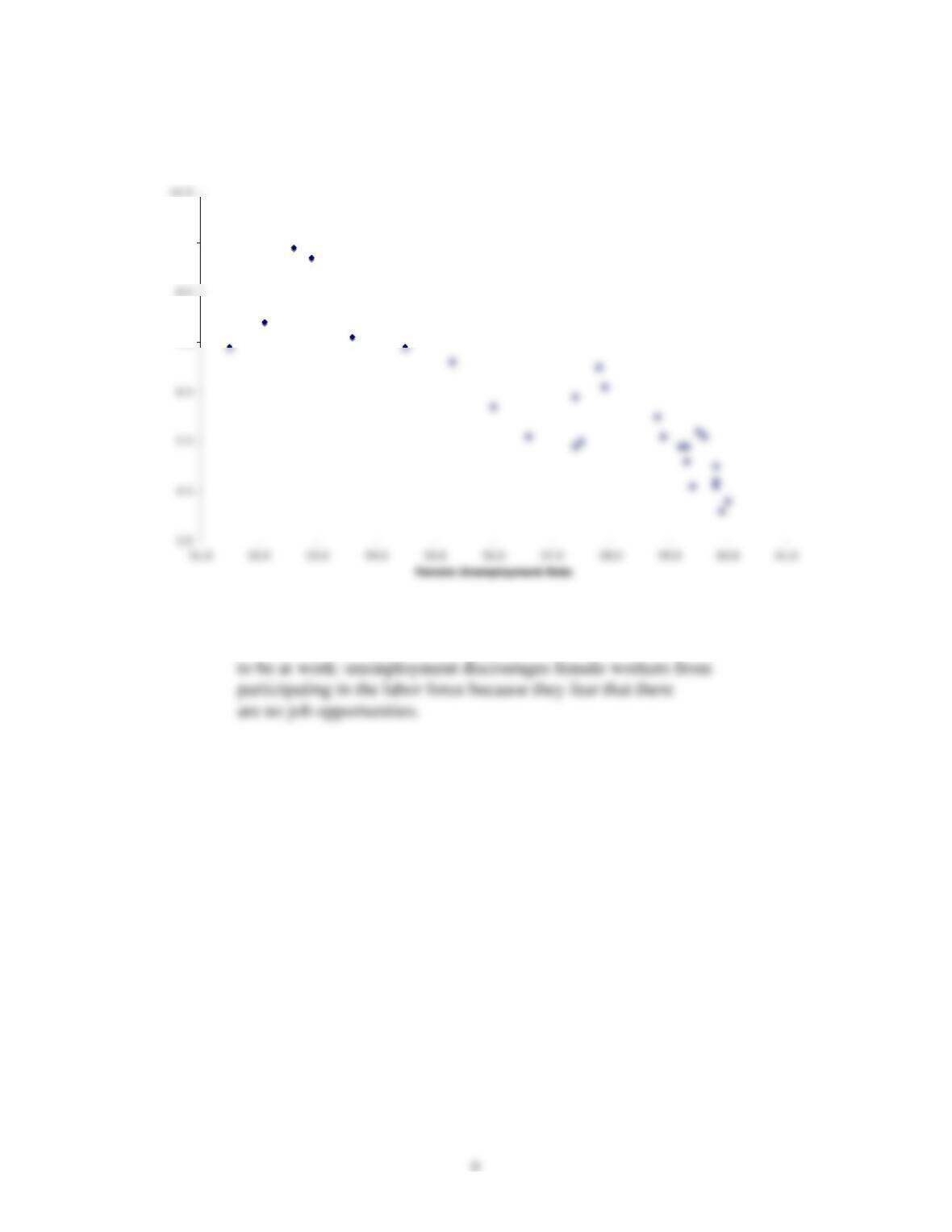
(b) The scattergram is as follows:
Here the discouraged worker hypothesis of labor economics seems
Female Labor Force Participation vs Unemployment Rate
7.5
9.5
Basic Econometrics, Gujarati and Porter
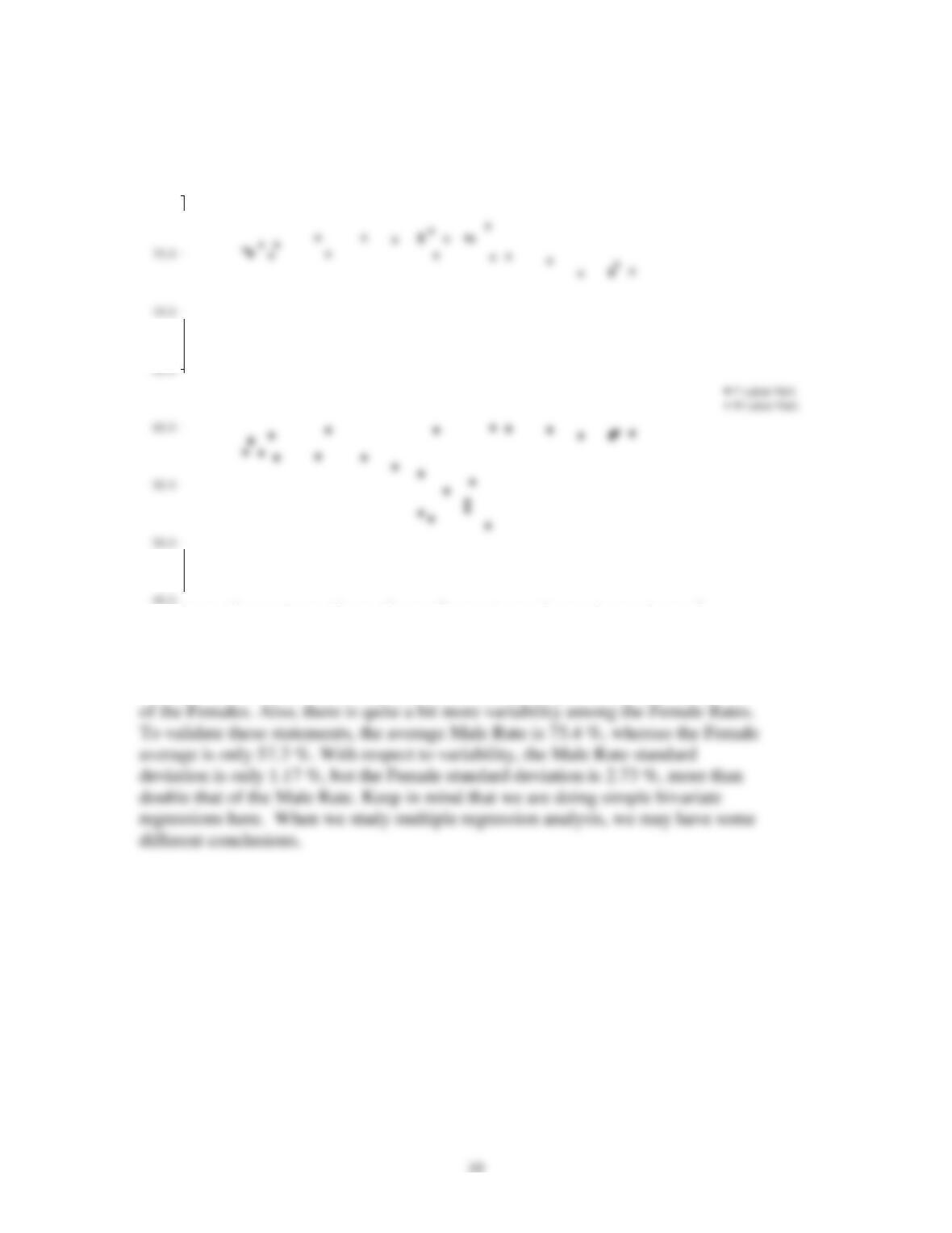
(c) The plot of Male and Female Labor Force Participation against
AH82 shows the following:
There is a similar relationship between the two variables for males and females,
although the Male Labor Participation Rate is always significantly higher than that
80.0
7.40 7.50 7.60 7.70 7.80 7.90 8.00 8.10 8.20 8.30 8.40
11
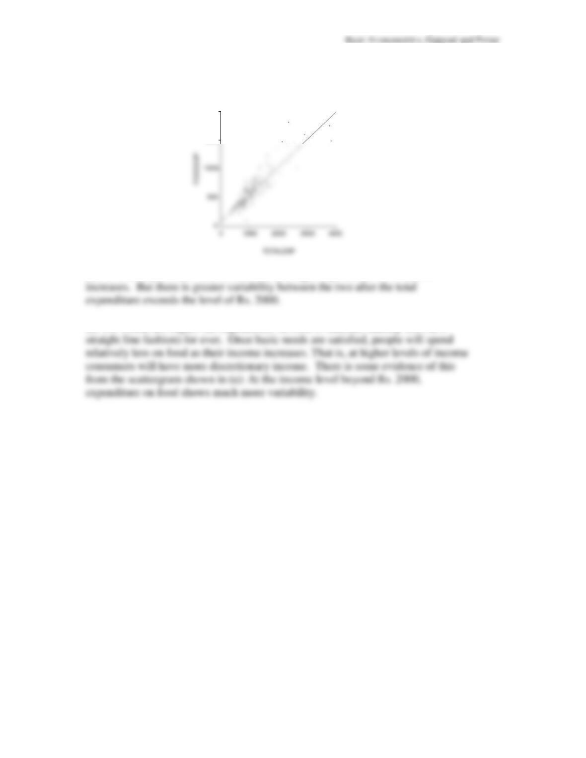
2.15 (a) The scattergram and the regression line look as follows:
(b) As total expenditure increases, on the average, expenditure on food also
(c) We would not expect the expenditure on food to increase linearly (i.e., in a
1500
2000
12
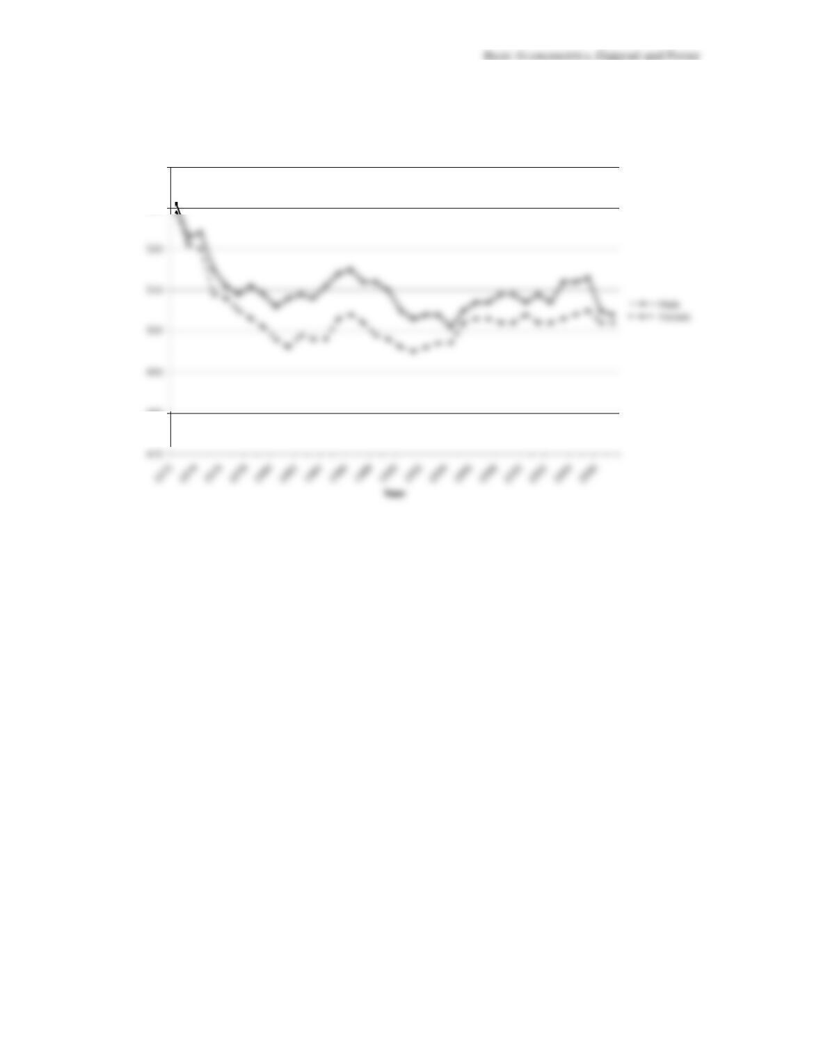
2.16 (a) The scatter plot for male and female verbal scores is as follows:
Male and Female Reading SAT Scores over Time
480
530
540
Basic Econometrics, Gujarati and Porter
13
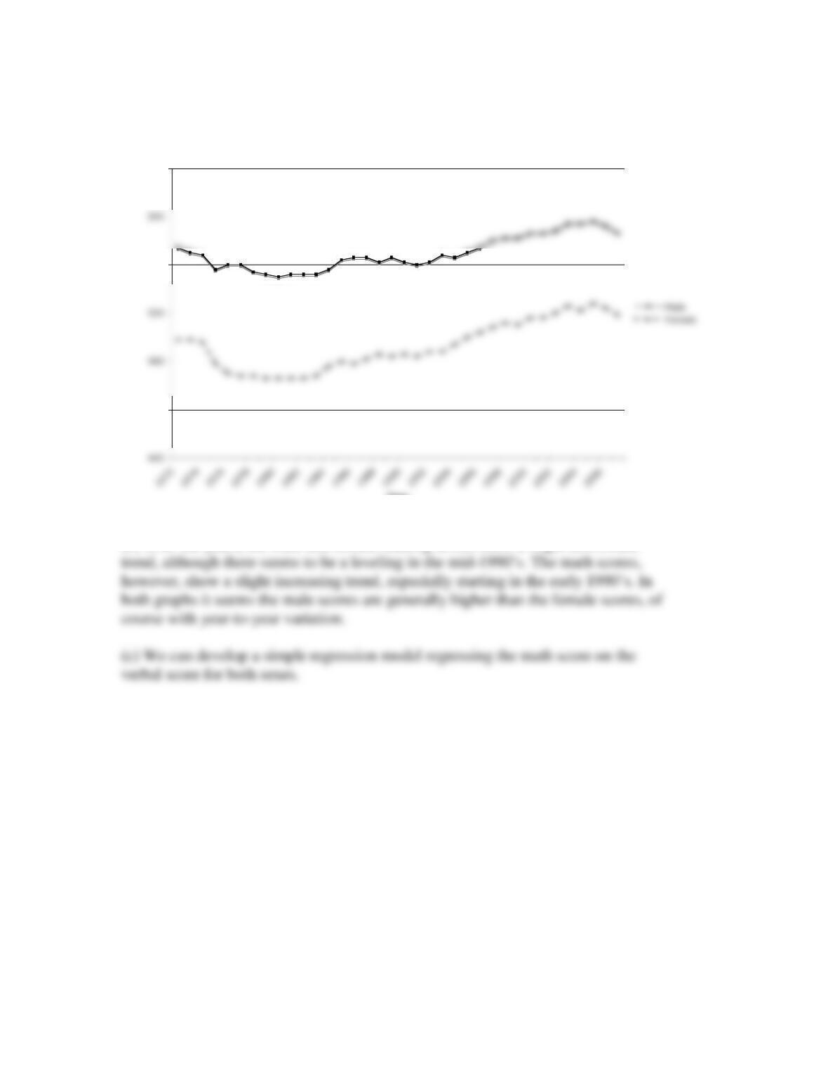
And the corresponding plot for male and female math score is as follows:
(b) Over the years, the male and female reading scores show a slight downward
Male and Female Math SAT Scores Over Time
460
520
560
Year
Basic Econometrics, Gujarati and Porter
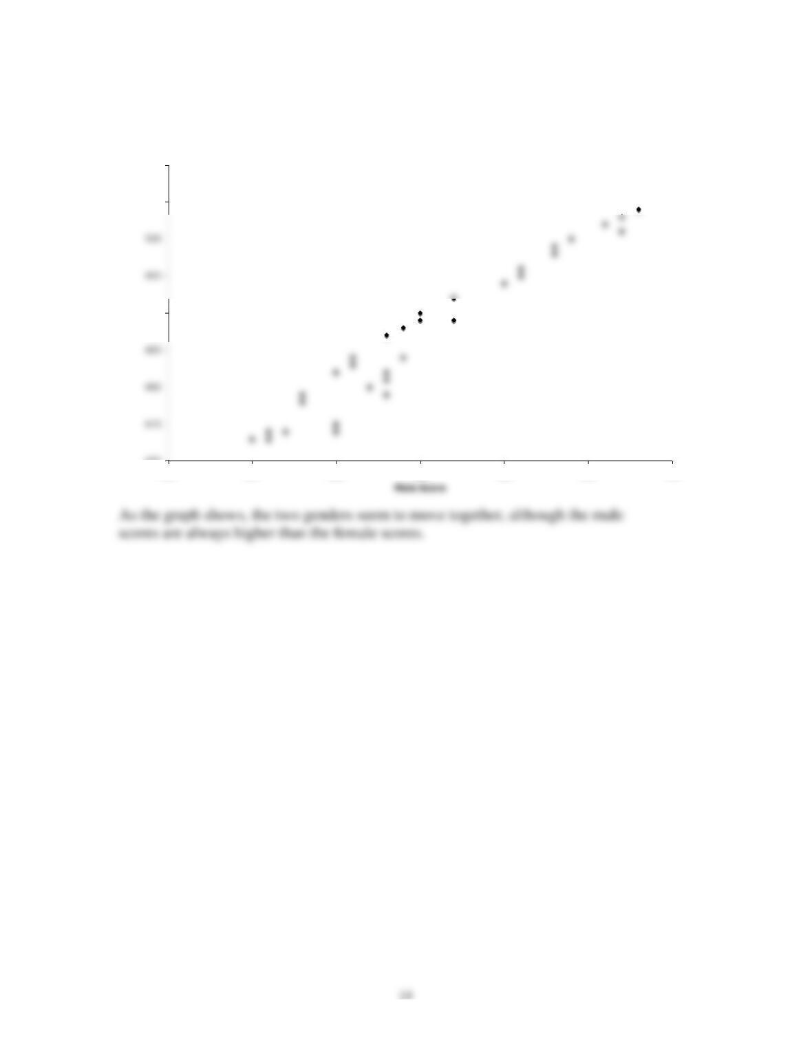
(d) The plot is as follows:
Female vs Male Math SAT Scores
470
490
505
510
510 515 520 525 530 535 540
15
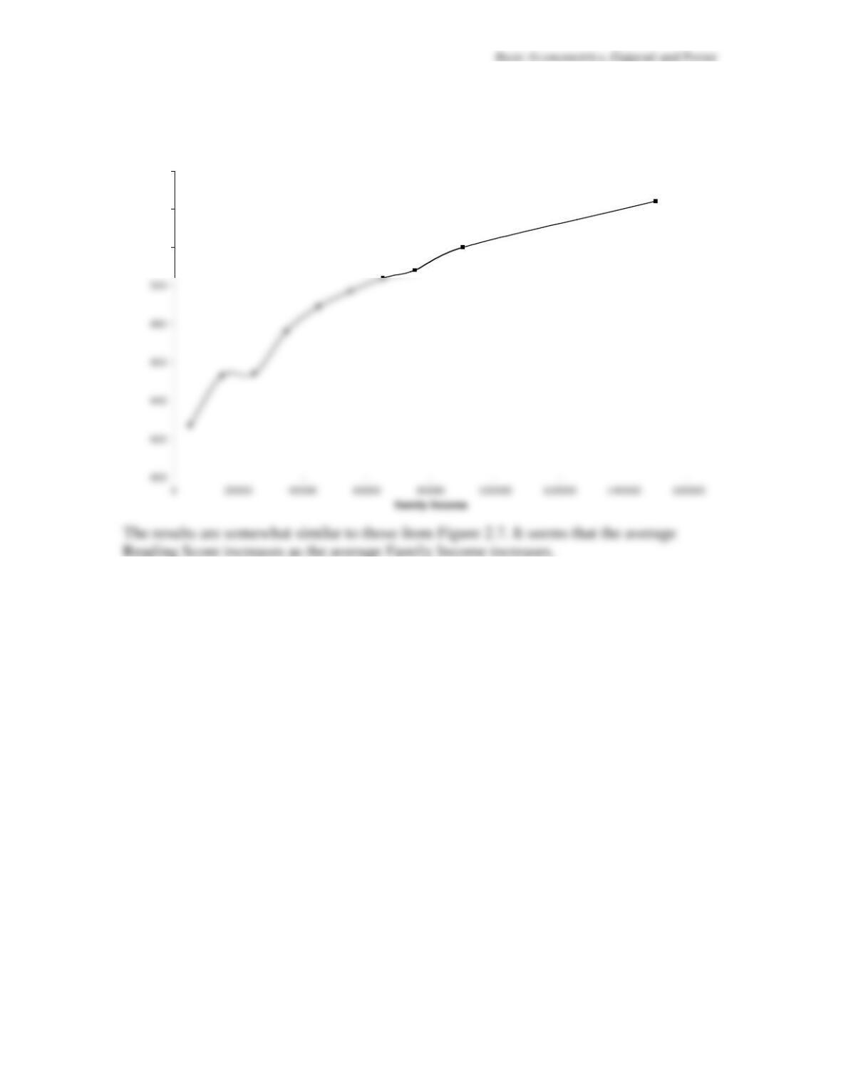
2.17 (a) The scatter plot for male and female verbal scores is as follows:
SAT Reading Scores vs Family Income
520
540
560
Basic Econometrics, Gujarati and Porter
16
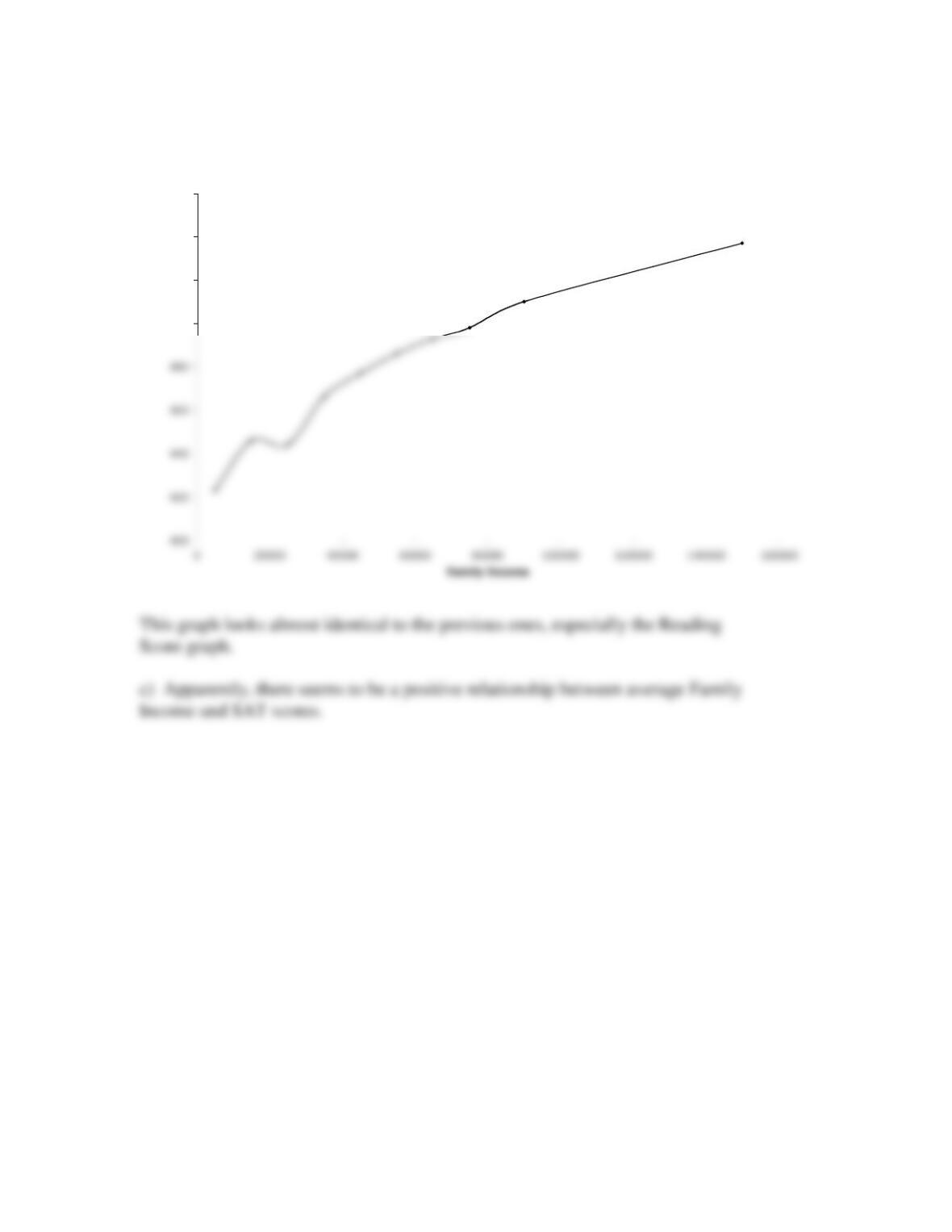
b)
SAT Writing Scores vs Family Income
500
520
540
560