CHAPTER 2
The Data of Macroeconomics
Notes to the Instructor
Chapter Summary
Chapter 2 is a straightforward chapter on economic data that emphasizes real GDP, the
Comments
Students may have seen this material in principles classes, so it can often be covered quickly. I
prefer not to get involved in the details of national income accounting; my aim is to get students
to understand the sort of issues that arise in looking at economic data and to know where to look
if and when they need more information. From the point of view of the rest of the course, the
most important things for students to learn are the identity of income and output, the distinction
between real and nominal variables, and the relationship between stocks and flows.
Use of the Web Site
The discussion of economic data can be made more interesting by encouraging students to use
the data plotter and look at the series being discussed. In using the software, the students should
Use of the Dismal Scientist Web Site
Use the Dismal Scientist Web site to download data for the past 40 years on nominal GDP and
the components of spending (consumption, investment, government purchases, exports, and
imports). Compute the shares of spending accounted for by each component. Discuss how the
shares have changed over time.
Chapter Supplements
This chapter includes the following supplements:
2-2 Nominal and Real GDP Since 1929
2-4 The Components of GDP (Case Study)
2-6 Seasonal Adjustment and the Seasonal Cycle
2-7 Measuring the Price of Light

2-9 CPI Improvements and the Decline in Inflation During the 1990s
2-11 Alternative Measures of Unemployment
2-12 Improving the National Accounts
Lecture Notes |
17
!Figure 2-1
!Figure 2-2
!
Lecture Notes
Introduction
An immense amount of economic data is gathered on a regular basis. Every day, newspapers,
radio, television, and the Internet inform us about some economic statistic or other. Although we
cannot discuss all these data here, it is important to be familiar with some of the most important
measures of economic performance.
2-1 Measuring the Value of Economic Activity: Gross Domestic Product
The single most important measure of overall economic performance is Gross Domestic Product
(GDP), which aims to summarize all economic activity over a period of time in terms of a single
number. GDP is a measure of the economy’s total output and of total income. Macroeconomists
Income, Expenditure, and the Circular Flow
Suppose that the economy produces just one good—bread—using labor only. (Notice what we
are doing here: We are making simplifying assumptions that are obviously not literally true to
gain insight into the working of the economy.) We assume that there are two sorts of economic
actors—households and firms (bakeries). Firms hire workers from the households to produce
bread and pay wages to those households. Workers take those wages and purchase bread from
the firms. These transactions take place in two markets—the goods market and the labor market.
FYI: Stocks and Flows
Goods are not produced instantaneously—production takes time. Therefore, we must have a
period of time in mind when we think about GDP. For example, it does not make sense to say a
bakery produces 2,000 loaves of bread. If it produces that many in a day, then it produces 4,000
in two days, 10,000 in a (five–day) week, and about 130,000 in a quarter. Because we always
have to keep a time dimension in mind, we say that GDP is a flow. If we measured GDP at any
tiny instant of time, it would be almost zero.
Rules for Computing GDP
Naturally, the measurement of GDP in the economy is much more complicated in practice than
our simple bread example suggests. There are any number of technical details of GDP
measurement that we ignore, but a few important points should be mentioned.
First, what happens if a firm produces a good but does not sell it? What does this mean for
GDP? If the good is thrown out, it is as if it were never produced. If one fewer loaf of bread is
18 | CHAPTER 2 The Data of Macroeconomics
!Supplement 2-3,
“Chain–Weighted
Real GDP”
!Supplement 8–5,
“Growth Rates,
Logarithms, and
Elasticities”
!Supplement 2-2,
“Nominal and
Real GDP Since
sold, then both expenditure and profits are lower. This is appropriate, since we would not want
GDP to measure wasted goods. Alternatively, the bread may be put into inventory to be sold
later. Then the rules of accounting specify that it is as if the firm purchases the bread from itself.
Both expenditure and profit are the same as if the bread were sold immediately.
Second, what happens if there is more than one good in the economy? We add up different
commodities by valuing them at their market price. For each commodity, we take the number
produced and multiply by the price per unit. Adding this over all commodities gives us total
GDP.
Many goods are intermediate goods—they are not consumed for their own sake but are
used in the production of other goods. Sheet metal is used in the production of cars; beef is used
in the production of hamburgers. The GDP statistics include only final goods. If a miller
produces flour and sells that flour to a baker, then only the final sale of bread is included in
Real GDP versus Nominal GDP
Valuing goods at their market price allows us to add different goods into a composite measure
but also means we might be misled into thinking we are producing more if prices are rising.
Thus, it is important to correct for changes in prices. To do this, economists value goods at the
The GDP Deflator
The GDP deflator is the ratio of nominal to real GDP:
Chain–Weighted Measures of Real GDP
In 1996, the Bureau of Economic Analysis changed its approach to indexing GDP. Instead of
using a fixed base year for prices, the Bureau began using a moving base year. Previously, the
Bureau used prices in a given year—say, 1990—to measure the value of goods produced in all
years. Now, to measure the change in real GDP from, say, 2014 to 2015, the Bureau uses the
prices in both 2014 and 2015. To measure the change in real GDP from 2015 to 2016, prices in
2015 and 2016 are used.
FYI: Two Arithmetic Tricks for Working with Percentage
Changes
The percentage change of a product in two variables equals (approximately) the sum of the
percentage changes in the individual variables. The percentage change of the ratio of two
Lecture Notes | 19
!Supplement 3–5,
“Economists’
Terminology”
“The Components
of GDP”
The Components of Expenditure
Although GDP is the most general measure of output, we also care about what this output is
used for. National income accounts thus divide total expenditure into four categories,
corresponding approximately to who does the spending, in an equation known as the national
income identity,
Y = C + I + G + NX,
where C is consumption, I is investment, G is government purchases, and NX is net exports, or
exports minus imports. Consumption is expenditure on goods and services by households; it is
thus the spending that individuals carry out every day on food, clothes, movies, DVD players,
automobiles, and the like. Food, clothing, and other goods that last for short periods of time are
Investment is for the most part expenditure by firms on factories, machinery, and
intellectual property products; this is known as business fixed investment. We noted earlier that
goods put into inventory by firms are counted as part of expenditure; they are classified as
inventory investment. This can be negative if firms are running down their stocks of inventory
rather than increasing them. A third component of investment spending is actually carried out by
households and landlords—residential fixed investment. This is the purchase of new housing.
The third category of expenditure corresponds to purchases by government (at all levels—
federal, state, and local). It includes, most notably, defense expenditures, as well as spending on
highways, bridges, and so forth. It is important to realize that it includes only spending on goods
FYI: What Is Investment?
Economists use the term “investment” in a very precise sense. To the economist, investment
means the purchase of newly created goods and services to add to the capital stock. It does not
apply to the purchase of already existing assets, since this simply changes the ownership of the
capital stock.
Case Study: GDP and Its Components
Other Measures of Income
There are other measures of income apart from GDP. The most important are as follows: gross
national product (GNP) equals GDP minus income earned domestically by foreign nationals
plus income earned by U.S. nationals in other countries; net national product (NNP) equals GNP
20 | CHAPTER 2 The Data of Macroeconomics
!Supplement 2–5,
“Defining National
Income”
!Supplement 2–6,
“Seasonal
Adjustment and the
Seasonal Cycle”
minus a correction for the depreciation or wear and tear of the capital stock (consumption of
fixed capital). The capital consumption allowance equaled about 16 percent of GNP in 2013. Net
national product is approximately equal to national income. The two measures differ by a small
amount known as the statistical discrepancy, which reflects differences in data sources that are
Seasonal Adjustment
Many economic variables exhibit a seasonal pattern—for example, GDP is lowest in the first
quarter of the year and highest in the last quarter. Such fluctuations are not surprising since some
sectors of the economy, such as construction, agriculture, and tourism, are influenced by the
weather and the seasons. For this reason, economists often correct for such seasonal variation
and look at data that are seasonally adjusted.
Case Study: The New, Improved GDP of 2013
An important change in how the Bureau of Economic Analysis calculates GDP occurred with the
2013 comprehensive revision of the national income and product accounts. This change
involves treating expenditures associated with creating intangible assets, such as artistic works
or research and development, in the same manner as tangible assets, such as machine tools or
factory buildings. Prior to this change, expenditures on intangible assets were treated as
2-2 Measuring the Cost of Living: The Consumer Price Index
We noted earlier the difference between real and nominal GDP: Real GDP takes GDP measured
in dollars—nominal GDP—and adjusts for inflation. There are two basic measures of the
inflation rate: the percentage change in the GDP deflator and the percentage change in the
consumer price index (CPI).
The Price of a Basket of Goods
The percentage change in the consumer price index is a good measure of inflation as it affects
the typical household. The CPI is calculated on the basis of a typical “basket of goods,” based on
a survey of consumers’ purchases. The point of having a basket of goods is that price changes
The CPI versus the GDP Deflator
The GDP deflator is a measure of the price of all goods produced in the United States that go
into GDP. In particular, the GDP deflator accounts for changes in the price of investment goods
and goods purchased by the government, which are not included in the CPI. It is, thus, a good
Lecture Notes | 21
!Supplement 2-7,
“Measuring the
Price of Light”
!Supplement 2-8,
“Improving the
CPI”
!Supplement 2-9,
measure of the price of “a unit of GDP.” The CPI is a poorer measure of the price of GDP, but it
provides a better measure of the price level as it affects the average consumer. Since the CPI
measures the cost of a typical set of consumer purchases, it does not include the prices of, say,
earthmoving equipment or Stealth bombers. It does include the prices of imported goods that
consumers purchase, such as Japanese televisions. Both of these factors make the CPI differ
from the GDP deflator.
Another measure of inflation is the implicit price deflator for personal consumption
expenditures, or PCE deflator. This measure, computed as the ratio of nominal consumption
expenditures to real consumption expenditures, is similar to the GDP deflator but includes only
the consumption component of GDP. Like the CPI, the PCE deflator excludes goods purchased
by government and by businesses and includes imported goods. Like the GDP deflator, it allows
the basket of goods to change over time. Because of these characteristics, the Federal Reserve
uses the PCE deflator as its preferred measure of inflation.
Does the CPI Overstate Inflation?
Many economists believe that changes in the CPI are an overestimate of the true inflation rate.
We already noted that the CPI overstates inflation because consumers substitute away from more
expensive goods. There are two other considerations.
• New Goods When producers introduce a new good, consumers have
more choices and can make better use of their dollars to satisfy their wants. Each dollar
will, in effect, buy more for an individual, so the introduction of new goods is like a
decrease in the price level. This value of greater variety is not measured by the CPI.
2-3 Measuring Joblessness: The Unemployment Rate
Finally, we consider the measurement of unemployment. Employment and unemployment
statistics are among the most watched of all economic data, for a couple of reasons. First, a well–
22 | CHAPTER 2 The Data of Macroeconomics
!Figure 2-4
!Supplement 8-6,
“Labor Force
Participation”
The Household Survey
The U.S. Bureau of Labor Statistics calculates the unemployment rate and other statistics that
economists and policymakers use to gauge the state of the labor market. These statistics are
where POP is the population, E is the employed, U is the unemployed, and NL is those not in the
labor force. Thus, we have
L = E + U,
where L is the labor force. The labor–force participation rate is the fraction of the population in
the labor force:
Case Study: Trends in Labor–Force Participation
Over the period 1950 to 2013, labor–force participation among women rose sharply, from 34
percent to 57 percent, while among men it has declined from 86 percent to 70 percent. Many
factors have contributed to the increase in women’s participation, including new technologies
such as clothes–washing machines, dishwashers, refrigerators, etc., which reduced the time
needed for household chores; fewer children per family; and changing social and political
attitudes toward women in the work force. For men, the decline has been due to earlier and
The Establishment Survey
In addition to asking households about their employment status, the Bureau of Labor Statistics
also separately asks business establishments about the number of workers on their payroll each
month. This establishment survey covers 160,000 businesses that employ over 40 million
workers. The survey collects data on employment, hours worked, and wages, and provides
breakdowns by industry and job categories. Employment as measured by the establishment
survey differs from employment as measured by the household survey for several reasons. First,
a self–employed person is reported as working in the household survey but does not show up on

2001. Over the period November 2001 to August 2003, the household survey showed an
2-4 Conclusion: From Economic Statistics to Economic Models
This chapter has explained how we measure real GDP, prices, and unemployment. These are
24
LECTURE SUPPLEMENT
2-1 Measuring Output
As discussed in the text, we can measure the value of national output either by adding up all of
the spending on the economy’s output of goods and services or by adding up all of the incomes
generated in producing output. This basic equivalence between output and income allows us to
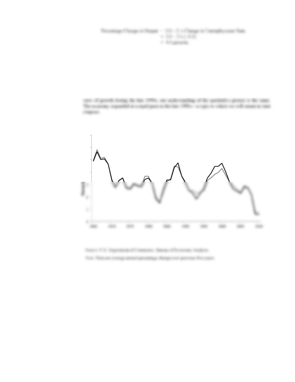
4.5 percent per year when measured using real GDI compared with 3.8 percent per year when
measured using real GDP. Figure 1 shows annual average growth rates over successive five–year
periods since 1960. As the figure illustrates, the difference in growth rates from the two
measures has typically averaged close to zero.
Which Measure Is More Accurate for the Mid– to Late 1990s?
Both the spending and income sides of the national accounts are measured with error because
significant portions of the data are estimates based on extrapolations from other indicators and
trends.1 As more complete data become available, the Bureau of Economic Analysis revises its
estimates of GDP and GDI. Generally, these annual and multiyear revisions replace more of the
spending–side estimates with detailed source data than the income–side estimates, which often
continue to be based on incomplete data. When tax returns and census data become available,
usually with a lag of many years, income estimates would be expected to improve. But because
these data for income remain far from complete, GDP would still be the more accurate measure,
25
just above the 3.8 percent growth rate of GDP. But, if we adjust Okun’s law for a (conservative)
0.5 percentage point step–up in long–run productivity growth during the mid– to late 1990s
(productivity growth is discussed in Chapter 9), then we obtain:
Percentage Change in Output = 3.5 – 2 × (-0.5) = 4.5 percent,
and Okun’s law would exactly match GDI growth rate of 4.5 percent.
Regardless of whether it is GDP or GDI that in the end turns out to provide a more accurate
Figure 1 Comparing Measures of Economic Growth
GDP$
GDI$
4$
5$
6$
7$
26
LECTURE SUPPLEMENT
2-2 Nominal and Real GDP Since 1929
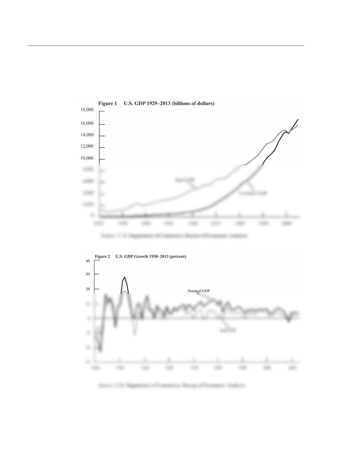
Figure 1 shows real GDP and nominal GDP between 1929 and 2013. Because real GDP is measured in
chained 2009 dollars, the two series intersect in 2009. Figure 2 examines the annual percentage change in
nominal and real GDP. Table 1 provides annual data for GDP and the GDP price index over the 1929–
2013 period.

Table 1 United States GDP: 1929–2013
Levels
Growth Rates
Year
Nominal GDP
(billions of
current
dollars)
Real GDP
(billions of
chained 2009
dollars)
GDP Price
Index
(2009 = 100)
Nominal
GDP
(percent)
Real GDP
(percent)
GDP Price
Index
(percent)
1929
104.6
1056.6
9.9
1930
92.2
966.7
9.5
–11.9
–8.5
–3.8
1931
77.4
904.8
8.6
–16.1
–6.4
–9.9
1932
59.5
788.2
7.6
–23.1
–12.9
–11.4
1933
57.2
778.3
7.4
–3.9
–1.3
–2.7
1934
66.8
862.2
7.8
16.8
10.8
4.9
1935
74.3
939.0
7.9
11.2
8.9
2.0
1936
84.9
1060.5
8.0
14.3
12.9
1.2
1937
93.0
1114.6
8.3
9.5
5.1
3.7
1938
87.4
1077.7
8.2
–6.0
–3.3
–1.8
1939
93.5
1163.6
8.0
7.0
8.0
–1.3
1940
102.9
1266.1
8.1
10.1
8.8
0.9
1941
129.4
1490.3
8.7
25.8
17.7
6.6
1942
166.0
1771.8
9.4
28.3
18.9
8.3
1943
203.1
2073.7
9.8
22.3
17.0
4.8
1944
224.6
2239.4
10.1
10.6
8.0
2.4
1945
228.2
2217.8
10.3
1.6
–1.0
2.5
1946
227.8
1960.9
11.6
–0.2
–11.6
12.6
1947
249.9
1939.4
12.9
9.7
–1.1
11.2
1948
274.8
2020.0
13.6
10.0
4.2
5.6
1949
272.8
2008.9
13.6
–0.7
–0.5
–0.1
1950
300.2
2184.0
13.7
10.0
8.7
0.9
1951
347.3
2360.0
14.7
15.7
8.1
6.8
1952
367.7
2456.1
15.0
5.9
4.1
2.2
1953
2571.4
15.2
6.0
4.7
1.3
1954
391.1
2556.9
15.3
0.4
–0.6
1.0
1955
426.2
2739.0
15.6
9.0
7.1
1.4
1956
450.1
2797.4
16.1
5.6
2.1
3.4
1957
474.9
2856.3
16.7
5.5
2.1
3.5
1958
482.0
2835.3
17.1
1.5
–0.7
2.3
1959
522.5
3031.0
17.3
8.4
6.9
1.3
1960
543.3
3108.7
17.5
4.0
2.6
1.4
1961
563.3
3188.1
17.7
3.7
2.6
1.1
1962
605.1
3383.1
17.9
7.4
6.1
1.2
1963
638.6
3530.4
18.1
5.5
4.4
1.1
1964
685.8
3734.0
18.4
7.4
5.8
1.5
1965
743.7
3976.7
18.7
8.4
6.5
1.8
1966
815.0
4238.9
19.3
9.6
6.6
2.8
1967
861.7
19.8
5.7
2.7
2.9
1968
942.5
4569.0
20.7
9.4
4.9
4.3
(Continued on next page)

28
Levels
Growth Rates
Year
Nominal GDP
(billions of
current dollars)
Real GDP
(billions of
chained 2005
dollars)
GDP Chain–
type Price
Index (2005 =
100)
Nominal
GDP
(percent)
Real GDP
(percent)
GDP Chain–
type Price
Index
(Percent)
1974
1548.8
5396.0
28.8
8.4
–0.5
9.0
1976
1877.6
5675.4
33.2
11.2
5.4
5.5
1977
2086.0
5937.0
35.2
11.1
4.6
6.2
1978
2356.6
6267.2
37.7
13.0
5.6
7.0
1979
2632.1
6466.2
40.8
11.7
3.2
8.3
1980
2862.5
6450.4
44.5
8.8
–0.2
9.0
1981
3211.0
6617.7
48.7
12.2
2.6
9.4
1982
3345.0
6491.3
51.6
4.2
–1.9
6.1
1983
3638.1
6792.0
53.7
8.8
4.6
3.9
1984
4040.7
7285.0
55.6
11.1
7.3
3.6
1985
4346.7
7593.8
57.3
7.6
4.2
3.2
1986
4590.2
7860.5
58.5
5.6
3.5
2.0
1987
4870.2
8132.6
59.9
6.1
3.5
2.4
1988
5252.6
8474.5
62.0
7.9
4.2
3.5
1989
5657.7
8786.4
64.4
7.7
3.7
3.9
1990
5979.6
8955.0
66.8
5.7
1.9
3.7
1991
6174.0
8948.4
69.1
3.3
–0.1
3.3
1992
6539.3
9266.6
70.6
5.9
3.6
2.3
1993
6878.7
9521.0
72.3
5.2
2.7
2.4
1994
7308.8
9905.4
73.9
6.3
4.0
2.1
1995
7664.1
10174.8
75.4
4.9
2.7
2.1
1996
8100.2
10561.0
76.8
5.7
3.8
1.8
1997
8608.5
11034.9
78.1
6.3
4.5
1.7
1998
9089.2
11525.9
78.9
5.6
4.4
1.1
1999
9660.6
12065.9
80.1
6.3
4.7
1.4
2000
10284.8
12559.7
81.9
6.5
4.1
2.3
2001
10621.8
12682.2
83.8
3.3
1.0
2.3
2002
10977.5
12908.8
85.0
3.3
1.8
1.5
2003
11510.7
13271.1
86.7
4.9
2.8
2.0
2004
12274.9
13773.5
89.1
6.6
3.8
2.7
2005
13093.7
14234.2
92.0
6.7
3.3
3.2
2006
13855.9
14613.8
94.8
5.8
2.7
3.1
2007
14477.6
14873.7
97.3
4.5
1.8
2.7
2008
14718.6
14830.4
99.2
1.7
–0.3
1.9
2009
14418.7
14418.7
100.0
–2.8
0.8
2010
14964.4
14783.8
101.2
3.8
2.5
1.2
2011
15517.9
15020.6
103.3
3.7
1.6
2.1
2012
16163.2
15369.2
105.2
4.2
2.3
1.8
2013
16768.1
15710.3
106.7
3.7
2.2
1.5
Source: U.S. Department of Commerce, Bureau of Economic Analysis.
1975
1688.9
5385.4
31.4
9.0
9.3
29
LECTURE SUPPLEMENT
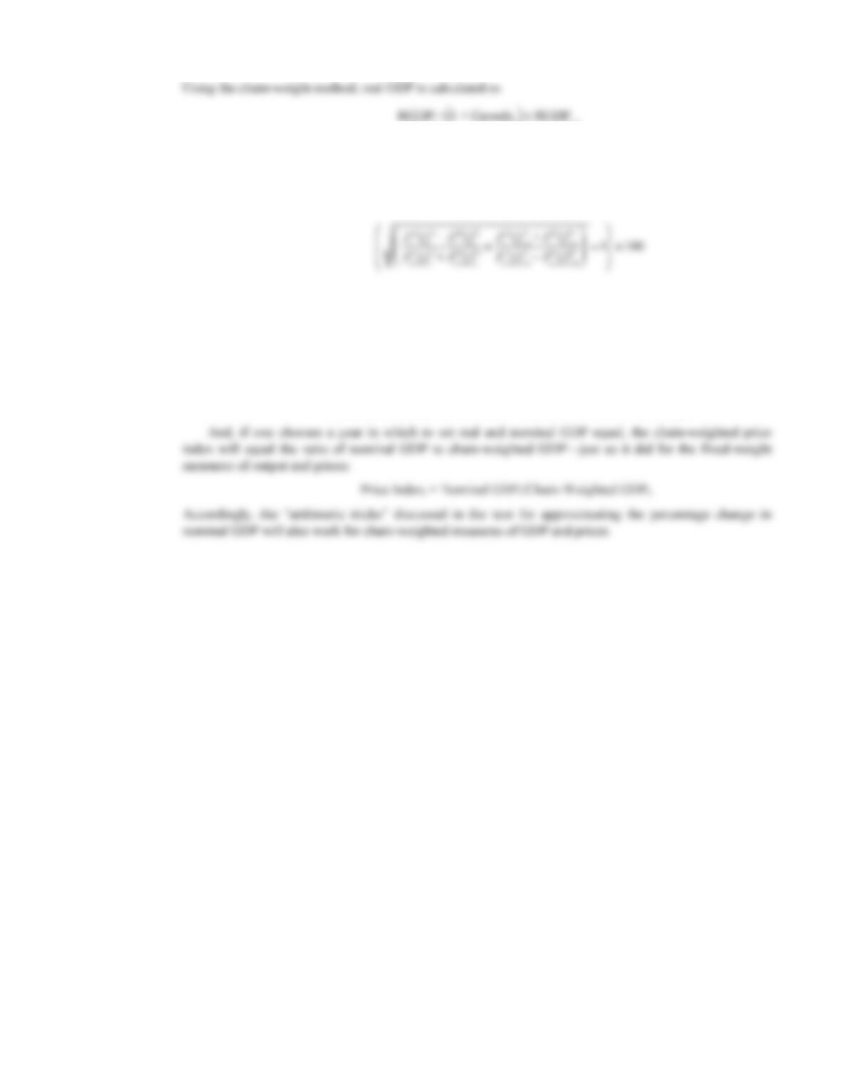
2-3 Chain–Weighted Real GDP
For nearly 50 years, the U.S. Bureau of Economic Analysis calculated real GDP and hence the growth rate
of the economy by valuing goods and services at the prices prevailing in a fixed year, known as the base
year. Most recently, 1987 was used as the base year. Thus, real GDP in 1995 was calculated by valuing all
goods and services produced in 1995 at the prices they sold for in 1987. Similarly, real GDP in 1950 was
Likewise, moving back in time over years prior to the base year, GDP growth is understated because those
goods and services with rapid output growth are underweighted compared to current prices and those
goods and services with slow output growth are overweighted.
The most widely cited example of substitution bias is computers. The price of computers (holding
quality fixed) has declined rapidly and the quantity produced has risen sharply. For example, the Bureau of
To reduce the extent of mismeasurement for recent years, the base year was updated every five years.
In 1991 the base year was changed from 1982 to 1987. Changing the base year, however, affects the
measurement of economic growth in all years. While moving the base year forward provides a more
accurate measurement of current growth, it worsens the underestimation of growth in early years.
In 1996, rather than updating the base year to 1992, the Bureau of Economic Analysis switched the
30
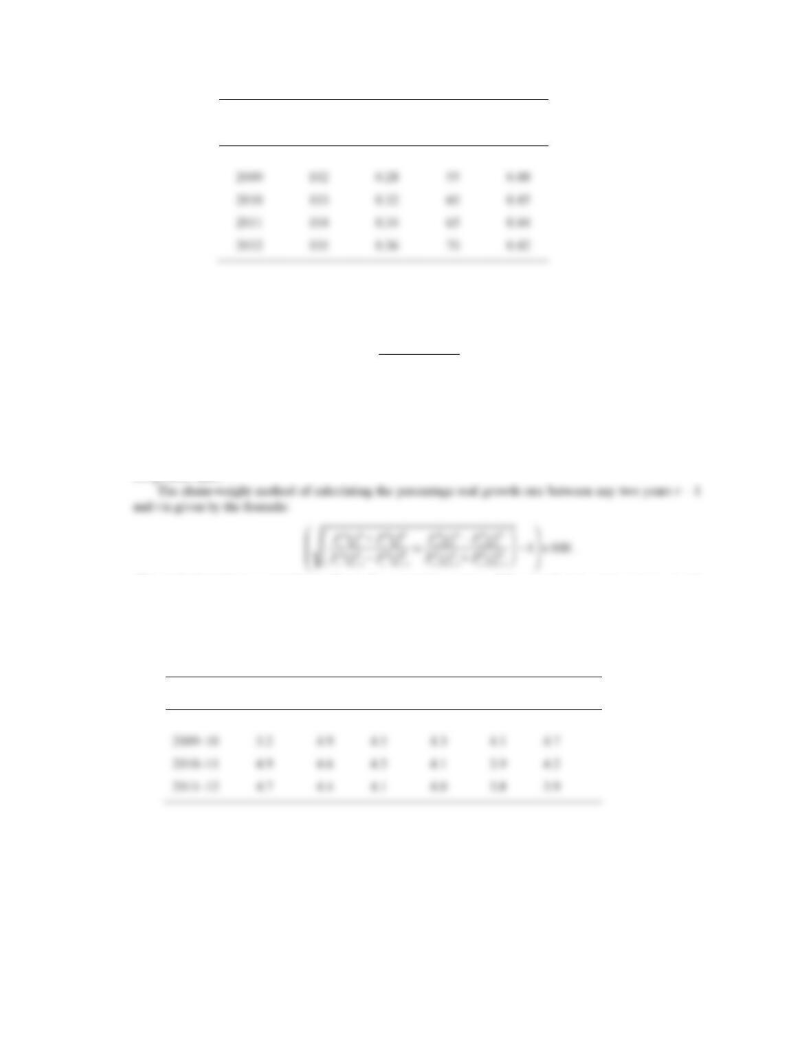
Table 1 Output and Prices of Apples and Oranges
Apples
Oranges
Year
Quantity
Price
Quantity
Price
2008
100
$0.25
50
$0.50
Table 2 calculates the growth rates of real GDP on a year–to–year basis from 2008 to 2012. Using a
fixed–weight measure, the percentage growth rate of real GDP from year t – 1 to year t is given by the
formula
,
where the superscript A refers to apples, the superscript O refers to oranges and the subscript B is the base
year. Columns 2–6 indicate how the year–to–year growth rates vary as the base year changes. For example,
the growth of real GDP between 2008 and 2009 varies from 4.9 percent to 6.0 percent depending on which
year is used as the base for prices. Note that the farther away from the base, the greater the difference in
growth rates. This explains why using 2008 prices or 2012 prices for the weights provides the extremes for
the growth rates.
This method produces a growth rate that is the geometric average of the growth rates using year t – 1 and
year t. The growth rate of real GDP between 2011 and 2012 was 4.0 percent using prices in 2011 for the
weights and 3.8 percent using prices in 2012 for the weights. The geometric average of these two growth
rates is 3.9 percent, the growth rate given by the chain–weight method.
Table 2 Growth Rate of Real Output Using Fixed–Weight or Chain–Weight Method
2008
Base
2009
Base
2010
Base
2011
Base
2012
Base
Chain–
Weight
2008–09
6.0%
5.7%
5.3%
5.1%
4.9%
5.8%
2010–11
4.9
4.6
4.3
4.1
3.9
4.2
2011–12
4.7
4.4
4.1
4.0
3.8
3.9
P
B
AQt
A+ P
B
OQt
O
P
B
AQt−1
A+ P
B
OQt−1
O−1
+100
2009
102
55
2011
104
65
2012
105
70
31
where growtht is the growth rate from year t – 1 to year t. Some year must be chosen for which real GDP is
set equal to nominal GDP (for U.S. GDP, the BEA currently uses 2009).
Calculating the chain–weight price index is similar to the process for calculating real GDP. The
percentage growth rate of prices in the apple and orange economy is given by:
The equation used to calculate the price index itself is:
Price Indext = (1 + Inflation Ratet) × Price Indext–1
where the inflation rate is the rate of change in prices from year t – 1 to year t.
The chain–weighted measures of real GDP and the price index also have the property that 1 plus the
growth of nominal GDP divided by 1 plus the growth of real GDP will equal 1 plus the inflation rate:
(1 + Inflation Ratet) = (1 + Growth Nominal GDPt)/(1 + Growtht).
( )