6
CHAPTER 2
TEACHING NOTES
This is the chapter where I expect students to follow most, if not all, of the algebraic derivations.
In class I like to derive at least the unbiasedness of the OLS slope coefficient, and usually I
derive the variance. At a minimum, I talk about the factors affecting the variance. To simplify
You might notice how, compared with most other texts, I use relatively few assumptions to
derive the unbiasedness of the OLS slope estimator, followed by the formula for its variance.
This is because I do not introduce redundant or unnecessary assumptions. For example, once
SLR.4 is assumed, nothing further about the relationship between u and x is needed to obtain the
unbiasedness of OLS under random sampling.
Incidentally, one of the uncomfortable facts about finite-sample analysis is that there is a
7
SOLUTIONS TO PROBLEMS
2.1 (i) Income, age, and family background (such as number of siblings) are just a few
possibilities. It seems that each of these could be correlated with years of education. (Income
2.2 In the equation y =
0 +
1x + u, add and subtract
0 from the right hand side to get y = (
0 +
2.3 (i) Let yi = GPAi, xi = ACTi, and n = 8. Then
x
= 25.875,
y
= 3.2125,
1
n
i=
(xi –
x
)(yi –
y
) =
The intercept does not have a useful interpretation because ACT is not close to zero for the
population of interest. If ACT is 5 points higher,
GPA
increases by .1022(5) = .511.
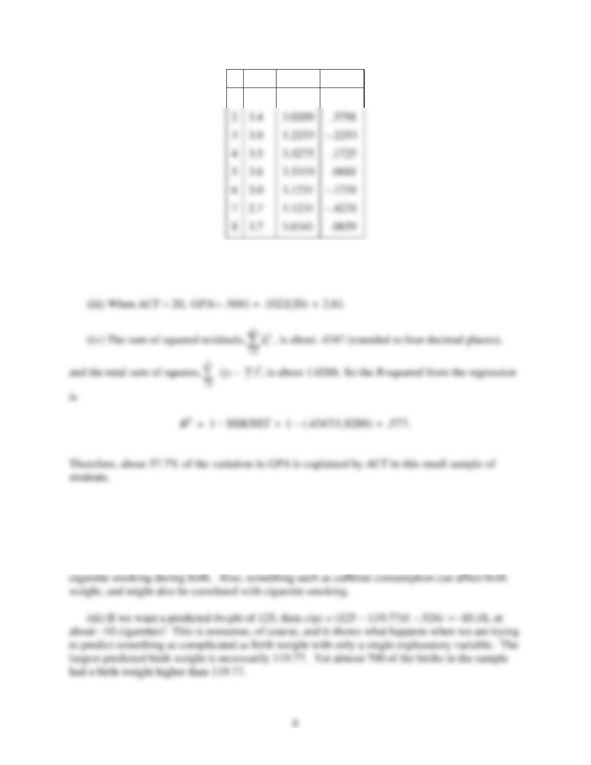
i
GPA
GPA
ˆ
u
1
2.8
2.7143
.0857
2
3.4
.3791
4
3.5
.1725
6
3.0
7
2.7
You can verify that the residuals, as reported in the table, sum to −.0002, which is pretty close to
zero given the inherent rounding error.
2.4 (i) When cigs = 0, predicted birth weight is 119.77 ounces. When cigs = 20,
bwght
= 109.49.
This is about an 8.6% drop.
(ii) Not necessarily. There are many other factors that can affect birth weight, particularly
overall health of the mother and quality of prenatal care. These could be correlated with
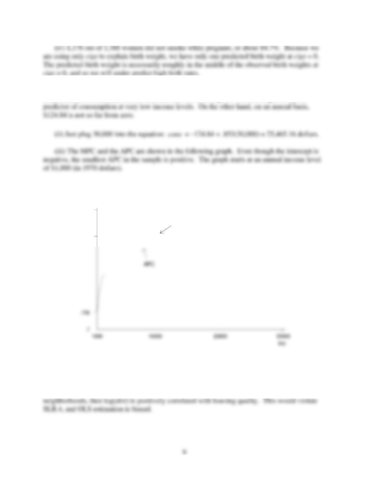
2.5 (i) The intercept implies that when inc = 0, cons is predicted to be negative $124.84. This, of
course, cannot be true, and reflects that fact that this consumption function might be a poor
2.6 (i) Yes. If living closer to an incinerator depresses housing prices, then being farther away
increases housing prices.
(ii) If the city chose to locate the incinerator in an area away from more expensive
.853
APC
MPC .9
MPC
10
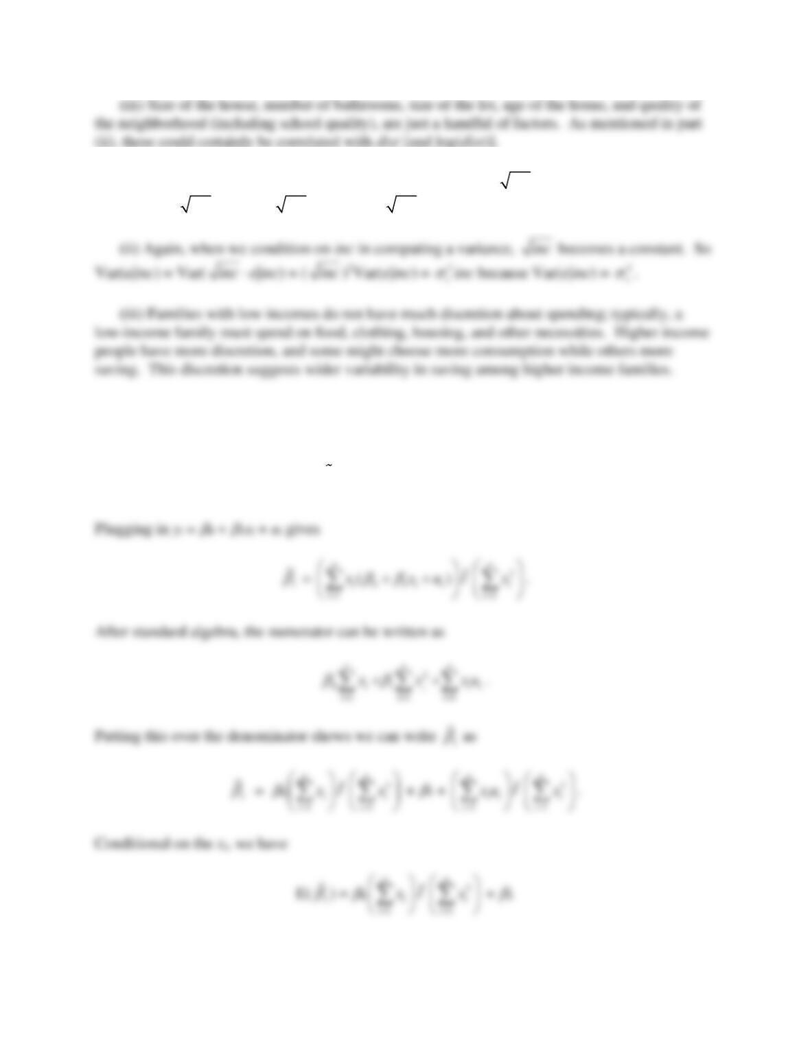
2.7 (i) When we condition on inc in computing an expectation,
inc
becomes a constant. So
E(u|inc) = E(
inc
e|inc) =
inc
E(e|inc) =
inc
inc
inc
inc
0 because E(e|inc) = E(e) = 0.
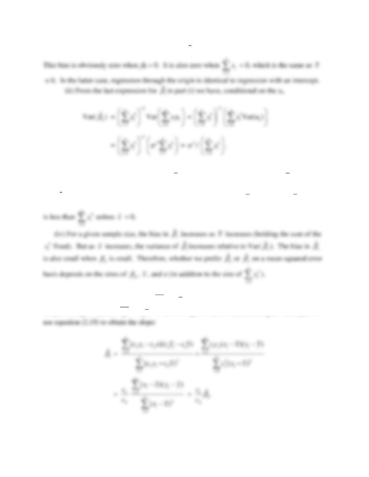
2.8 (i) From equation (2.66),
1
=
1
n
ii
i
xy
=
/
2
1
n
i
i
x
=
2
1
n
i
i
x
=
2
1
n
i
i
x
=
.
11
because E(ui) = 0 for all i. Therefore, the bias in
1
is given by the first term in this equation.
(iii) From (2.57), Var(
1
ˆ
) =
2/
2
1
()
n
i
i
xx
=
−
. From the hint,
2
1
n
i
i
x
=
2
1
()
n
i
i
xx
=
−
, and so
Var(
1
) Var(
1
ˆ
). A more direct way to see this is to write
2
1
()
n
i
i
xx
=
−
=
22
1
()
n
i
i
x n x
=
−
, which
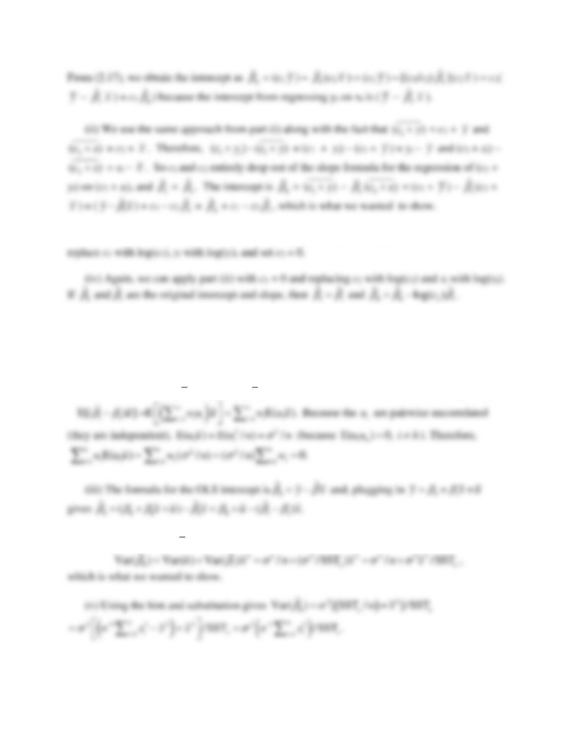
2.9 (i) We follow the hint, noting that
1
cy
=
1
cy
(the sample average of
1i
cy
is c1 times the
sample average of yi) and
cx
=
cx
. When we regress c1yi on c2xi (including an intercept) we
12
(iii) We can simply apply part (ii) because
11
log( ) log( ) log( )
ii
c y c y=+
. In other words,
2.10 (i) This derivation is essentially done in equation (2.52), once
(1/SST )
x
is brought inside
the summation (which is valid because
SSTx
does not depend on i). Then, just define
/SST
i i x
wd=
.
(ii) Because
1 1 1
ˆˆ
Cov( , ) E[( ) ] ,uu
=−
we show that the latter is zero. But, from part (i),
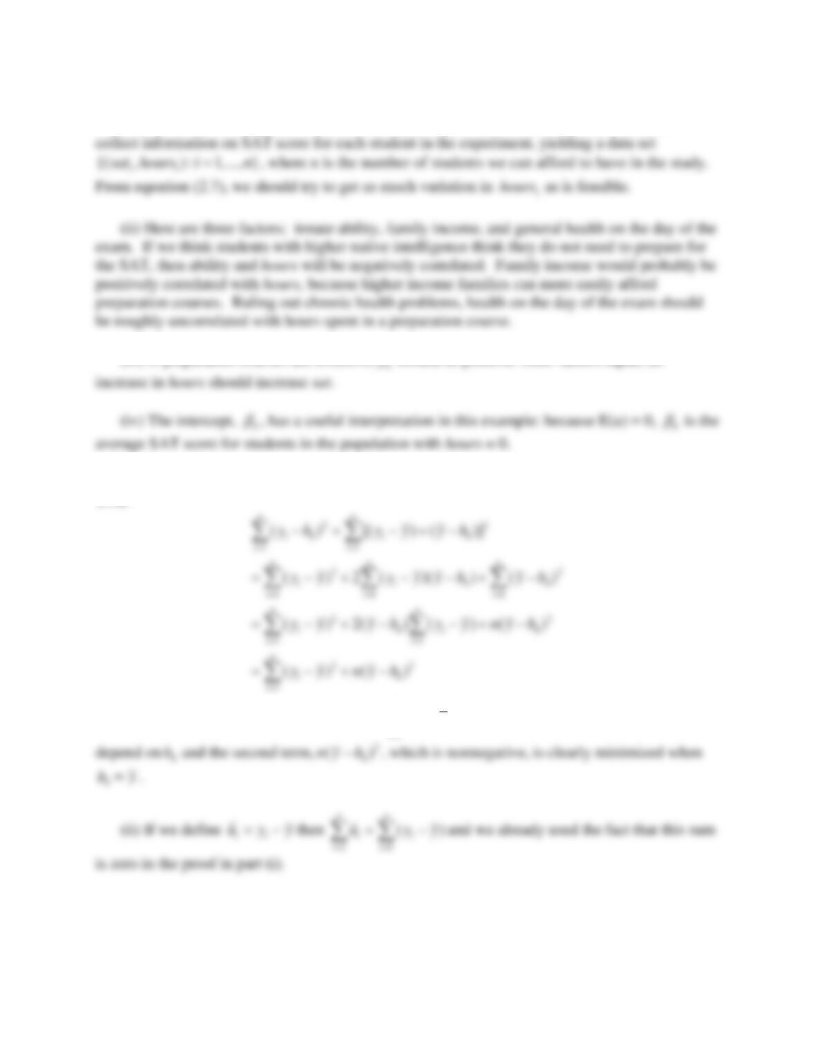
(iv) Because
1
ˆ and u
are uncorrelated,
13
2.11 (i) We would want to randomly assign the number of hours in the preparation course so that
hours is independent of other factors that affect performance on the SAT. Then, we would
(iii) If preparation courses are effective,
should be positive: other factors equal, an
2.12 (i) I will show the result without using calculus. Let 𝑦̅ be the sample average of the 𝑦𝑖 and
write
where we use the fact (see Appendix A) that
1
( ) 0
n
i
i
yy
=
−=
always. The first term does not
SOLUTIONS TO COMPUTER EXERCISES
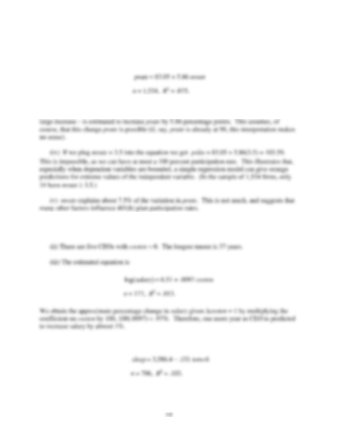
C2.1 (i) The average prate is about 87.36 and the average mrate is about .732.
(ii) The estimated equation is
(iii) The intercept implies that, even if mrate = 0, the predicted participation rate is 83.05
percent. The coefficient on mrate implies that a one-dollar increase in the match rate – a fairly
C2.2 (i) Average salary is about 865.864, which means $865,864 because salary is in thousands
of dollars. Average ceoten is about 7.95.
C2.3 (i) The estimated equation is
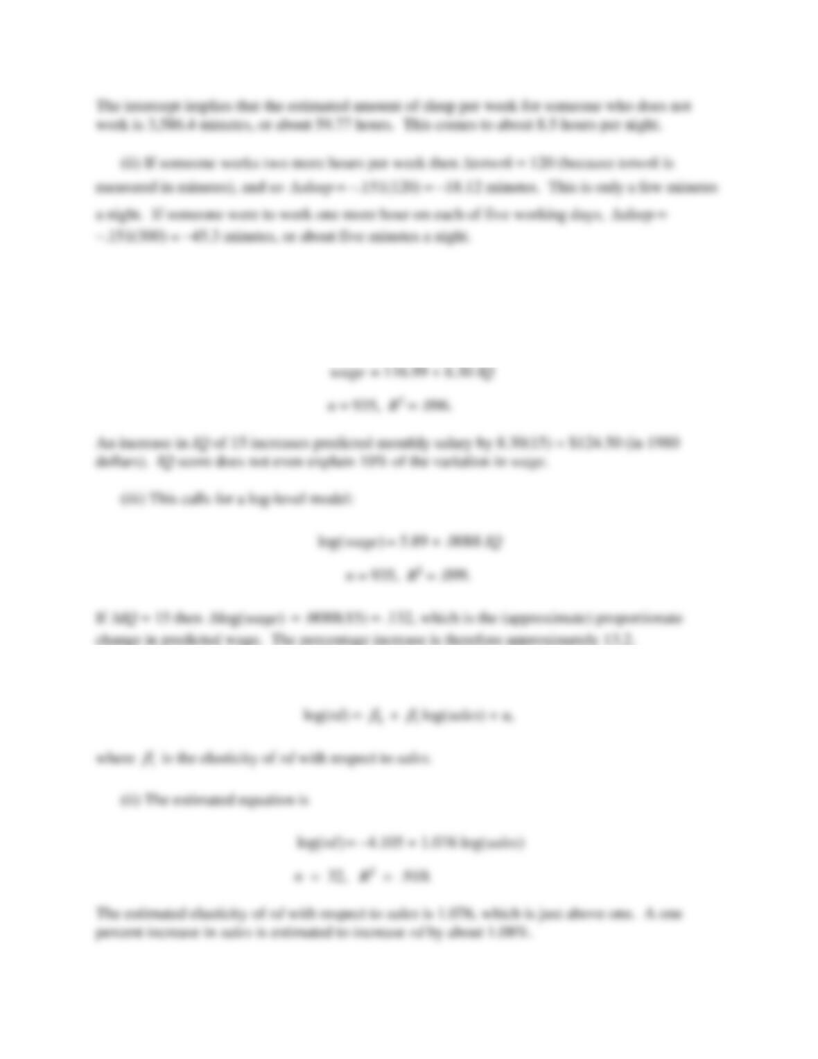
15
C2.4 (i) Average salary is about $957.95 and average IQ is about 101.28. The sample standard
deviation of IQ is about 15.05, which is pretty close to the population value of 15.
(ii) This calls for a level-level model:
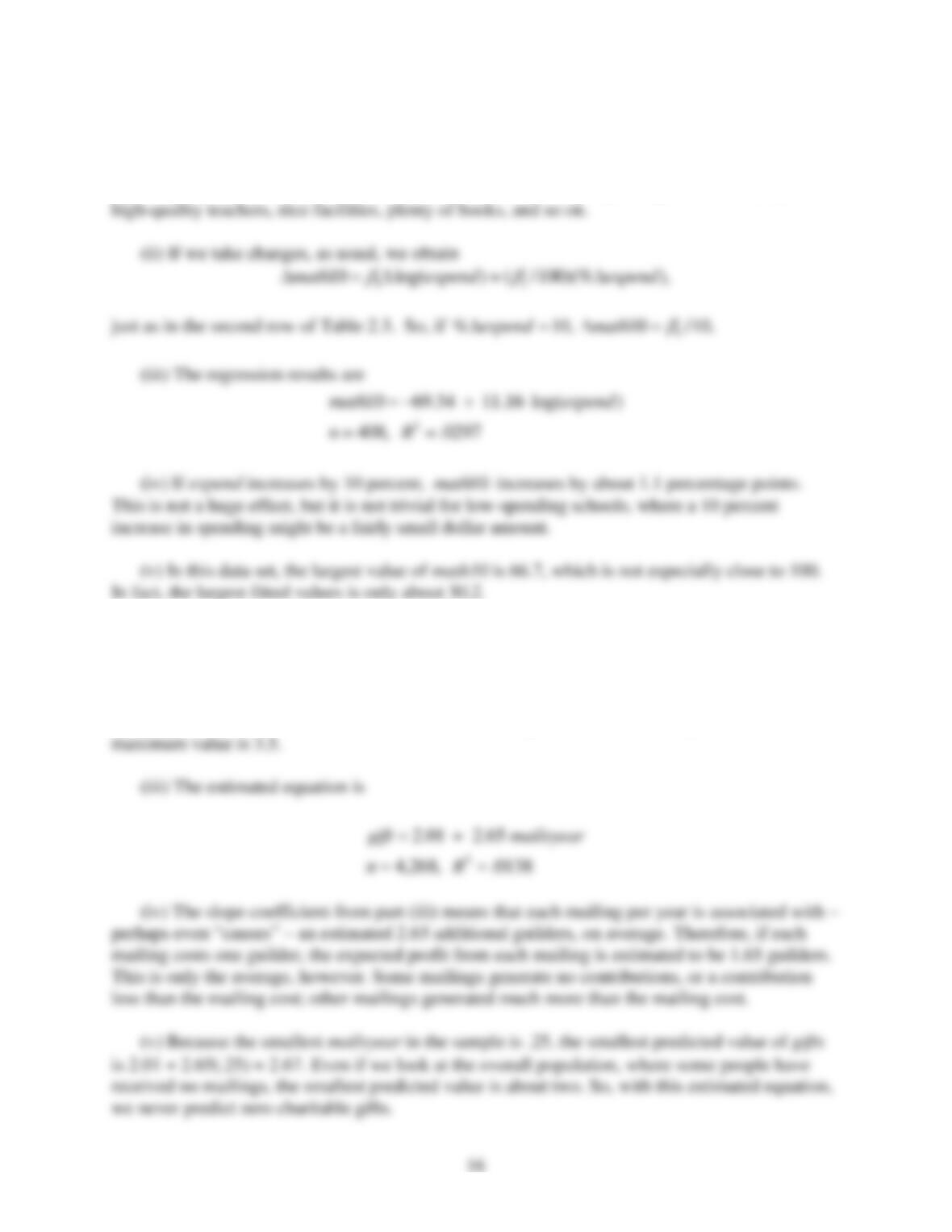
C2.5 (i) The constant elasticity model is a log-log model:
log(rd) =
C2.6 (i) It seems plausible that another dollar of spending has a larger effect for low-spending
schools than for high-spending schools. At low-spending schools, more money can go toward
purchasing more books, computers, and for hiring better qualified teachers. At high levels of
spending, we would expend little, if any, effect because the high-spending schools already have
C2.7 (i) The average gift is about 7.44 Dutch guilders. Out of 4,268 respondents, 2,561 did not
give a gift, or about 60 percent.
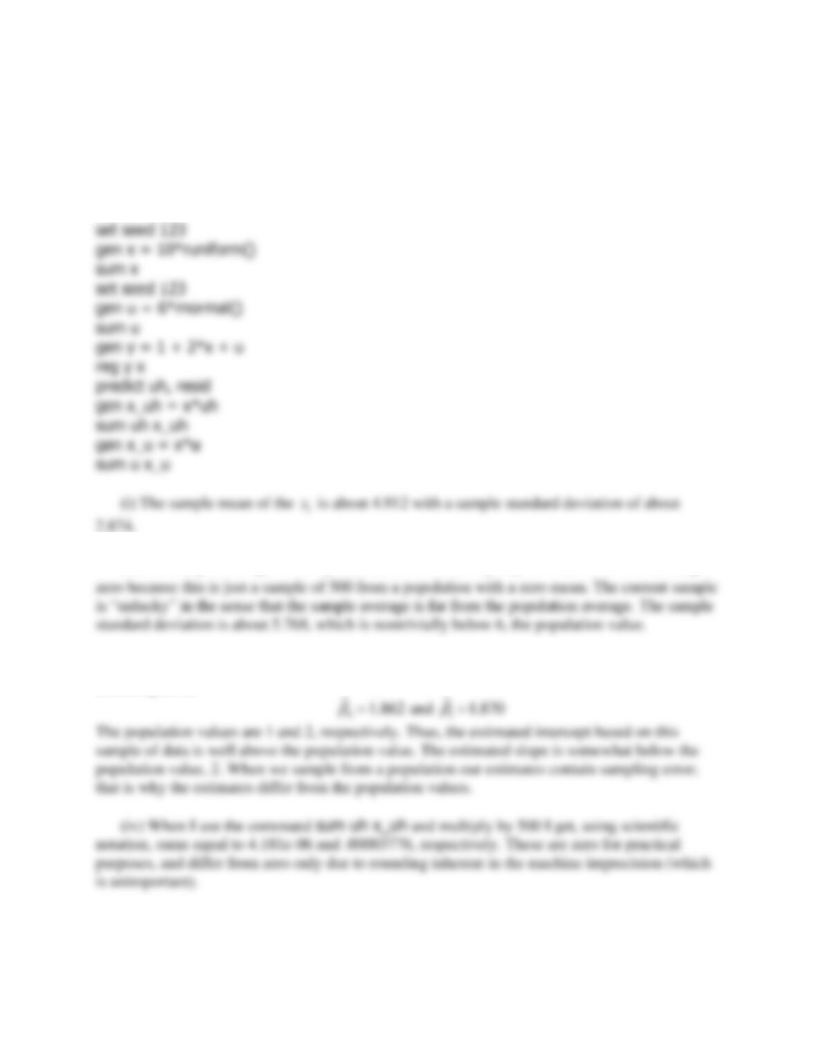
(ii) The average mailings per year is about 2.05. The minimum value is .25 (which
presumably means that someone has been on the mailing list for at least four years) and the
17
C2.8 There is no “correct” answer to this question because all answers depend on how the
random outcomes are generated. I used Stata 11 and, before generating the outcomes on the
i
x
, I
set the seed to the value 123. I reset the seed to 123 to generate the outcomes on the
i
u
.
Specifically, to answer parts (i) through (v), I used the sequence of commands
set obs 500
(ii) The sample average of the
i
u
is about .221, which is pretty far from zero. We do not get
(iii) After generating the data on
i
y
and running the regression, I get, rounding to three
decimal places,
18
(v) We already computed the sample average of the
i
u
in part (ii). When we multiply by 500
the sample average is about 110.74. The sum of
ii
xu
is about 6.46. Neither is close to zero, and
nothing says they should be particularly close.
i
u