Economics Chapter 19 In 2015 National Income In The United States Was $15,665.3 Billion

Unlock access to all the studying documents.

View Full Document

interactive activity

Chapter 19

Factor Markets and

the Distribution of Income

1. In 2015, national income in the United States was $15,665.3 billion. In the

same year, 148.8 million workers were employed, at an average wage, including

benefits, of $62,187 per worker per year.

a. How much compensation of employees was paid in the United States in 2015?

b. Analyze the factor distribution of income. What percentage of national income

was received in the form of compensation to employees in 2015?

c. Suppose that a huge wave of corporate downsizing leads many terminated

employees to open their own businesses. What is the effect on the factor distri-

bution of income?

59.1%.

c. The effect of this change is to diminish the share of income going to compen-

2. Marty’s Frozen Yogurt has the production function per day shown in the accom-

panying table. The equilibrium wage rate for a worker is $80 per day. Each cup

of frozen yogurt sells for $2.

Quantity of labor

(workers)

Quantity of frozen

yogurt (cups)

0 0

1110

a. Calculate the marginal product of labor for each worker and the value of the

marginal product of labor per worker.

b. How many workers should Marty employ?

S-270 Chapter 19 Factor Markets and the distribution oF incoMe

2. a. The accompanying table shows the marginal product of labor (MPL) and the

value of the marginal product of labor (VMPL) of each worker. Remember that

VMPL = P × MPL. Here that means that VMPL = $2 × MPL.

Quantity of labor

(workers)

Quantity of frozen

yogurt (cups)

MPL

(cups per worker)

VMPL

(per worker)

0 0

110 $220

1110

90 180

2200

70 140

b. Marty should employ 3 workers. The value of the marginal product of the

third worker ($140) is above the wage rate of $80: Marty should hire the third

3. The production function for Patty’s Pizza Parlor is given in the table in Problem 12.

3. The accompanying diagram shows the value of the marginal product of labor

curve and the wage rates of $10 and $15. As the wage rate increases from $10 to

$15, Patty’s demand for workers decreases from 2 workers to 1 worker. So, as the

wage rate increases, Patty should hire fewer workers.

10 2345

$18

Wage

rate

Quantity of labor (workers)

New wage

rate

Solution

4. Jameel runs a driver education school. The more driving instructors he hires,

the more driving lessons he can sell. But because he owns a limited number of

training automobiles, each additional driving instructor adds less to Jameel’s

output of driving lessons. The accompanying table shows Jameel’s production

function per day. Each driving lesson can be sold at $35 per hour.

Quantity of labor

(driving instructors)

Quantity of driving

lessons (hours)

0 0

1 8

Determine Jameel’s labor demand schedule (his demand schedule for driving

instructors) for each of the following daily wage rates for driving instructors:

$160, $180, $200, $220, $240, and $260.

4. The accompanying table calculates the marginal product of labor (MPL) and the

value of the marginal product of labor (VMPL).

Quantity of labor

(driving instructors)

Quantity of driving

lessons (hours)

MPL (hours per

driving instructor)

VMPL (per driving

instructor)

0 0

8 $280

1 8

If the daily wage rate of driving instructors is $160, Jameel should hire 4 instruc–

tors: the fourth instructor has a value of the marginal product of $175, which

is greater than the wage rate; but the fifth instructor would have a value of the

marginal product of only $140, which is less than the wage rate. By similar rea-

soning for the other wage rates, Jameel’s demand schedule for labor is as shown

in the accompanying table.

Daily wage rate

Quantity of labor

demanded (driving

instructors)

$160 4

260 1

Solution

5. Dale and Dana work at a self-service gas station and convenience store. Dale

opens up every day, and Dana arrives later to help stock the store. They are both

$9.50. This implies that all other workers hired will have an hourly value of the

marginal product higher than $9.50 but will be paid a wage of $9.50. Or to put it

6. A New York Times article observed that the wage of farmworkers in Mexico was

$11 an hour but the wage of immigrant Mexican farmworkers in California was

$9 an hour.

a. Assume that the output sells for the same price in the two countries. Does this

imply that the marginal product of labor of farmworkers is higher in Mexico

b. Now suppose that farmwork in Mexico is more arduous and more dangerous

than farmwork in California. As a result, the quantity supplied of labor for

any given wage rate is not the same for Mexican farmworkers as it is for immi-

6. a. We know that farmworkers are employed up to the point where the value of

the marginal product of labor is just equal to the wage: VMPL = P × MPL = W.

In Mexico, this means that P × MPLMexico = $11 and in California P ×

Solution

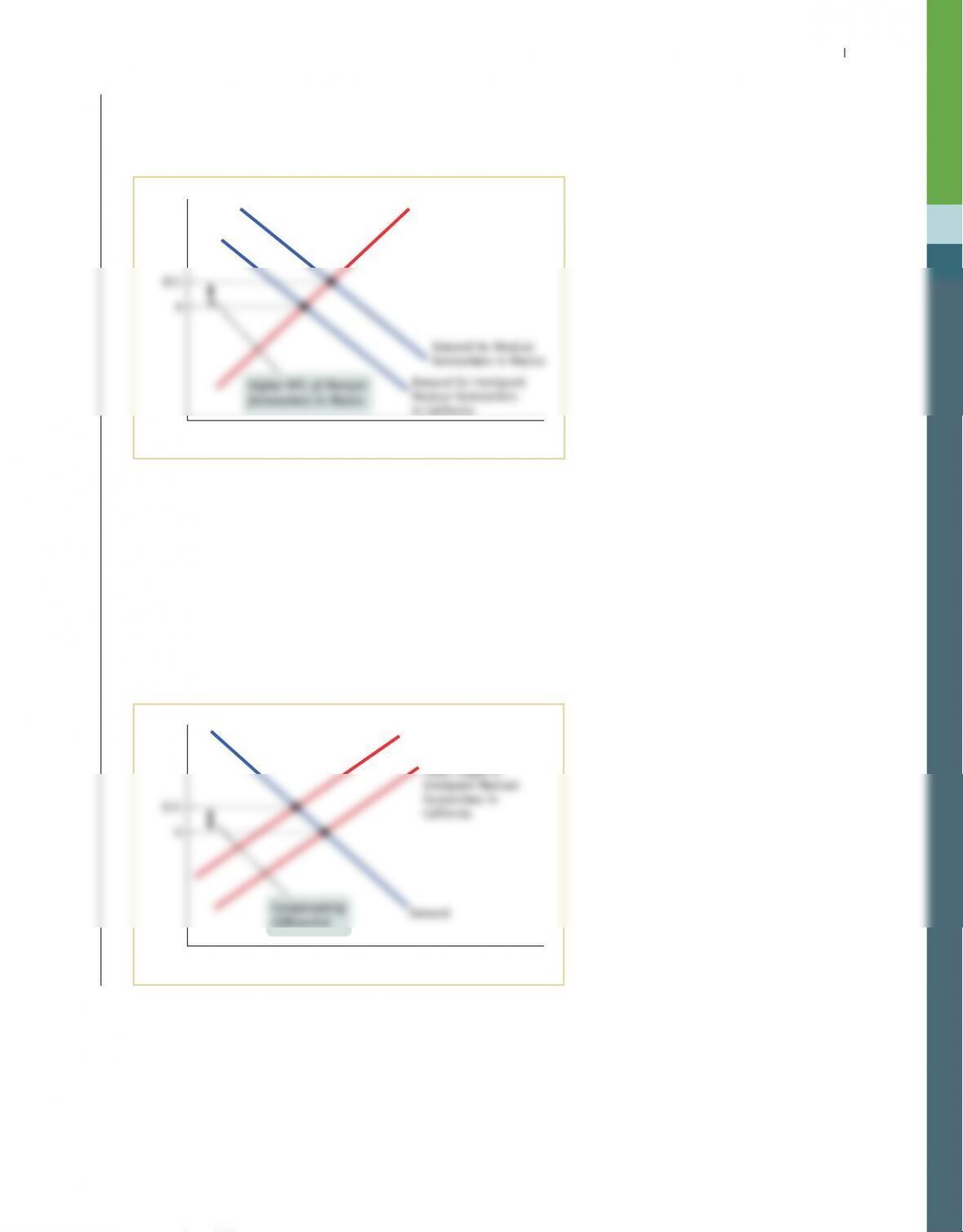
Chapter 19 Factor Markets and the distribution oF incoMe S-273

of workers is a result of differences in the demand curves for labor. Because

Mexican farmworkers have a higher marginal product of labor, the demand

curve for their labor lies above and to the right of the demand curve for their

peers in California, as shown in the accompanying diagram.

Supply

Wage

Quantity of labor

b. Because farmwork in Mexico is more arduous and dangerous than farmwork

in California, we can no longer infer that the higher wages paid to Mexican

farmworkers is evidence that they have a higher marginal product of labor

than their peers in California. Rather, the difference in wages is a compensat–

ing differential that compensates Mexican farmworkers for the greater diffi-

culty and danger they face.

c. Assuming that the quantity of labor demanded for any given wage rate is the

same for the two groups means that one demand curve can be drawn to repre-

sent employers’ demand responses in both markets. The compensating differ-

ential that Mexican farmworkers demand relative to their peers in California

is illustrated by their supply curve of labor in the accompanying diagram,

which lies above and to the left of the supply curve of their Californian peers.

Labor supply of Mexican

farmworkers in Mexico

Wage

Quantity of labor

S-274 Chapter 19 Factor Markets and the distribution oF incoMe

7. Kendra is the owner of Wholesome Farms, a commercial dairy. Kendra employs

labor, land, and capital. In her operations, Kendra can substitute between the

amount of labor she employs and the amount of capital she employs. That is, to

produce the same quantity of output she can use more labor and less capital;

similarly, to produce the same quantity of output she can use less labor and

more capital. Let w* represent the annual cost of labor in the market, let r

represent the annual cost of a unit of land in the market, and let rK

* represent

the annual cost of a unit of capital in the market.

a. Suppose that Kendra can maximize her profits by employing less labor and

more capital than she is currently using but the same amount of land. What

three conditions must now hold for Kendra’s operations (involving her value of

the marginal product of labor, land, and capital) for this to be true?

8. For each of the following situations in which similar workers are paid different

wages, give the most likely explanation for these wage differences.

9. Research consistently finds that despite nondiscrimination policies, African–

American workers on average receive lower wages than White workers do. What

are the possible reasons for this? Are these reasons consistent with marginal

productivity theory?

10. Greta is an enthusiastic amateur gardener and spends a lot of her free time

working in her yard. She also has a demanding and well-paid job as a freelance

11. You are the governor’s economic policy adviser. The governor wants to put in

place policies that encourage employed people to work more hours at their jobs

and that encourage unemployed people to find and take jobs. Assess each of

11. a. The effect of this policy on the incentive to work is ambiguous. A lower income

tax rate has the effect of raising workers’ wages in a real sense. The substitu-

tion effect will induce people to work more, but the income effect will induce

them to work less. So this is an effective policy only if the substitution effect is

stronger than the income effect.

b. The effect of this policy on the incentive to work is also ambiguous. A higher

income tax rate has the effect of reducing workers’ wages in a real sense. The

WORK IT OUT Interactive step-by-step help with solving this

problem can be found online.

12. Patty’s Pizza Parlor has the production function per hour shown in the

accompanying table. The hourly wage rate for each worker is $10. Each pizza

sells for $2.

Quantity of labor

(workers) Quantity of pizza

0 0

1 9

a. Calculate the marginal product of labor for each worker and the value of

the marginal product of labor per worker.

b. Draw the value of the marginal product of labor curve. Use your diagram

to determine how many workers Patty should employ.

Now let’s assume that Patty buys a new high-tech pizza oven that allows her

workers to become twice as productive as before. That is, the first worker

now produces 18 pizzas per hour instead of 9, and so on.

Solution

12. a. The accompanying table shows the marginal product of labor (MPL) and the

value of the marginal product of labor (VMPL1).

Number of

workers

Quantity

of pizza

MPL

(pizzas per worker)

VMPL1 (per

worker) (price of

pizza = $2)

VMPL2 (per

worker) (price

of pizza = $4)

0 0

9$18 $36

1 9

612 24

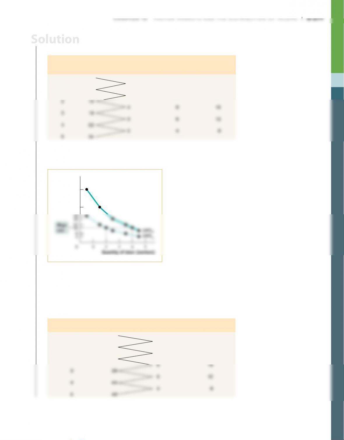
b. The accompanying diagram shows the value of the marginal product of labor

curve (VMPL1). The value of the marginal product of labor equals the wage

rate at 2 workers. So Patty should employ 2 workers.

$36

Wage

rate

Quantity of labor (workers)

c. The table shows the new value of the marginal product of labor (VMPL2). The

value of the marginal product of labor curve is labeled VMPL2 in the diagram.

The new value of the marginal product of labor equals the wage rate at 4

workers. So Patty should employ 4 workers.

d. The accompanying table shows the new production function for Patty’s Pizza

Parlor, the new marginal product of labor (MPL3), and the new value of the

marginal product of labor (VMPL3).

Quantity of labor

(workers)

Quantity of

pizza

MPL3 (pizzas per

worker) VMPL3 (per worker)

0 0

18 $36

118

12 24

230

Solution

S-278 Chapter 19 Factor Markets and the distribution oF incoMe

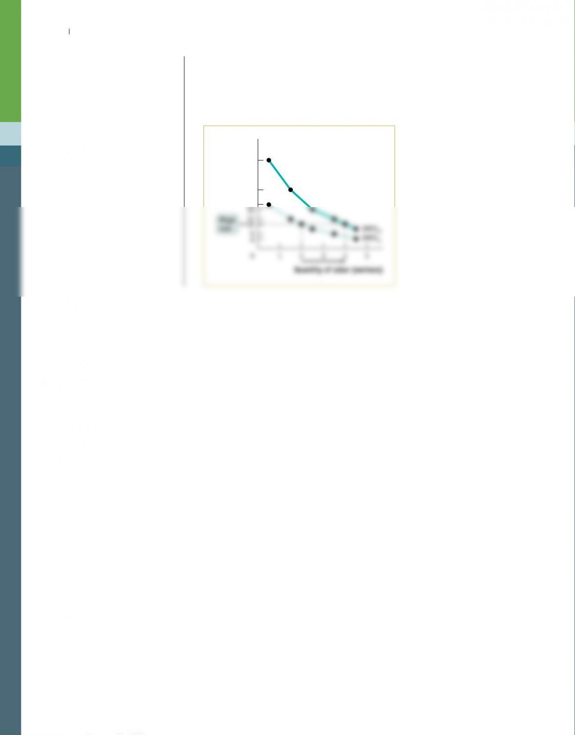
e. The accompanying diagram shows the original value of the marginal product

of labor curve from part b (VMPL1) and the new value of the marginal product

of labor curve (VMPL3). The value of the marginal product of labor now equals

the wage rate at 4 workers. So Patty should employ 4 workers. As the value of

the marginal product of labor increases—in this case as a result of a techno–

logical innovation (the new pizza oven)—Patty should hire more workers.

$36

Wage

rate

Quantity of labor

(

workers

)