CHAPTER 19
Government Debt and Budget
Deficits
Notes to the Instructor
Chapter Summary
This chapter begins with an analysis of the size of the U.S. government debt and the outlook for
the debt. It then discusses problems in accurately measuring the deficit and the debt. The last
Comments
As with the material on stabilization policy in Chapter 18, students find the study of government
debt to be quite relevant for understanding the debates concerning economic policy that are
frequently covered in the news media. The chapter includes a section that discusses balanced
budgets and optimal fiscal policy—helping students understand why deficits might sometimes
be beneficial. The case study about the fiscal future considers the reasons behind the troubling
long–term budget outlook. The chapter also introduces the role of debt in recent financial crises,
a topic covered more completely in Chapter 20.
Use of the Dismal Scientist Web Site
Go to the Dismal Scientist Web site and download annual data over the past 20 years for the
GDP price index and the federal debt outstanding (in the Flow of Funds data). Compute the
inflation rate from the GDP price index. Use the inflation rate along with the debt outstanding to
compute the component of interest on the debt that is due to inflation. Now download the federal
government budget deficit over the past 20 years. Subtract the inflation component from the
deficit to arrive at an adjusted deficit. Assess how this adjustment changes the pattern of the
deficit over this period.
Chapter Supplements
This chapter includes the following supplements:
19–2 How Important Is Crowding Out? (Case Study)
19-3 Structural and Cyclical Deficits
19-5 The Government Budget Constraint
19-6 Borrowing Constraints Using the Fisher Diagram

19-8 Is Everything Neutral?
19-9 Does Altruism Matter? (Case Study)
19–10 Unpleasant Monetarist Arithmetic
19–12 Additional Readings
Lecture Notes | 455
Lecture Notes
Introduction
One important controversy in macroeconomics concerns the role and significance of government
debt. Government deficits and government debt moved to the forefront of U.S. economic and
political debate in the 1980s, as the federal government increased its debt at a rate unprecedented
19–1 The Size of the Government Debt
The net debt of the U.S. federal government was nearly 86 percent of GDP in 2014. This was
well below the 143 percent share of GDP for Japan’s debt but larger than the 3.5 percent share
of GDP for Australia’s debt. Relative to other countries, the U.S. debt is roughly in the middle
of the pack. Another way to view its size is to note that in 2014, the $12.9 trillion debt held by
the public amounted to $41,000 for each of the 316 million people in the United States. Given
that the average person’s lifetime earnings are about $2 million, a per capita debt of $41,000
does not appear overwhelming.
Another important feature of the debt is that over time its size has fluctuated greatly. Debt
has typically risen during wars and fallen during peacetime. At the end of World War II, for
Case Study: The Troubling Outlook for Fiscal Policy
The long–term budget outlook is distressing. According to the Congressional Budget Office
(CBO), spending on programs for the elderly over the next several decades is projected to
increase more rapidly than the revenues supporting these programs, leading to rising deficits
and, thus, an accumulating federal debt. In particular, spending on Social Security, Medicare,
and Medicaid has risen from less than 1 percent of GDP in 1950 to about 10 percent today and
19–2 Problems in Measurement
Some disagreements about fiscal policy arise because of difficulties in obtaining an accurate and
economically meaningful measure of the deficit. There are many subtleties and arcane details of
!Table 19-1
!Figure 19-1
!Supplement 19–1,
“Debt and Deficits:
The Data”
!Supplement 19–2,
“How Important Is
456 | CHAPTER 19 Government Debt and Budget Deficits
Measurement Problem 1: Inflation
The deficit as usually measured is not adjusted for inflation. Part of the deficit is interest
payments on the government debt. By the Fisher equation, these interest payments equal iD = (r
+ π)D. The real interest payments are equal to rD, so the deficit is overstated by an amount equal
to πD. When inflation is high, this overstatement can be large: In 1979, for example, inflation
was 8.6 percent and the debt was $495 billion, implying that the deficit was overstated by about
$43 billion. Corrected for inflation, the reported budget deficit of $28 billion turns into a budget
surplus of $15 billion.
Measurement Problem 2: Capital Assets
The government’s budget deficit, as usually measured, accounts only for changes in the
government’s liabilities and not for changes in the government’s assets. Thus, if the government
were to sell a national park to developers and use the revenue to reduce its debt (liabilities), the
budget deficit would be lower. In this case, however, the reduction in the deficit does not mean
Measurement Problem 3: Uncounted Liabilities
Certain liabilities of the government, such as government employee pensions and accumulated
Social Security benefits, are excluded in calculation of the deficit. This is a particular problem in
the case of contingent liabilities, such as federal deposit insurance, that are paid only if certain
prespecified events (for example, a bank failure) occur.
Measurement Problem 4: The Business Cycle
Automatic changes in the deficit occur due to the direction in which the economy is going.
During a recession, for example, the budget deficit rises due to depressed tax revenue and
Summing Up
These measurement problems make the task of assessing government fiscal policy difficult. The
only safe lesson is that any simple statistic, such as the government deficit, provides only one
19–3 The Traditional View of Government Debt
We begin our theoretical analysis with a discussion of the standard IS–LM view of the deficit.
An increase in the deficit means either lower taxes or else increases in government expenditures
or transfer payments. All of these imply higher spending, either directly or through their effect
on disposable income. Hence, increases in the deficit are expansionary and are associated with
!Supplement 19–3,
“Structural and
!Supplement 19–4,
“Generational
457
IS and LM curves.
In the long run, after price adjustment returns the economy to full employment, we find
further crowding out. Increases in the price level reduce the real money supply, pushing interest
rates and the exchange rate up further and thus further decreasing investment and net exports. In
the long run, we see complete crowding out: Private spending is reduced by an amount exactly
equal to the increased government spending.
FYI: Taxes and Incentives
The textbook represents the tax system with a single variable, T, treating taxes as a simple lump–
sum amount. But in reality, we need to consider how tax revenue is actually raised. The field of
public finance spends a good deal of time addressing the benefits and costs of alternative types
of taxes. An important conclusion is that taxes have effects on economic incentives. When
people are taxed on income from working, they have less incentive to work, and when they are
taxed on income from capital, they have less incentive to invest. Accordingly, changes in taxes
19–4 The Ricardian View of Government Debt
There is not universal agreement on this reasoning. Some economists have argued that the logic
behind the IS–LM model is substantially flawed and that we should not expect to see crowding
out, nor should we expect to see deficits having any substantial impact on the economy. The
main argument is known as Ricardian equivalence, so named because the basic idea was first
noted by the nineteenth–century British economist David Ricardo. The current role of this theory
in macroeconomic debate is principally the result of work by economist Robert Barro.
The Basic Logic of Ricardian Equivalence
Ricardian equivalence argues that the effects on the economy are the same whether government
expenditures are financed by taxes or by borrowing (hence the term “equivalence”). Stated
differently, Ricardian equivalence argues that a debt–financed tax cut should have no effect on
the economy. This is in stark contrast to the standard view, in which the two types of financing
are not equivalent at all. The essence of this argument is that consumers understand the
Consumers and Future Taxes
For Ricardian equivalence to hold, consumers must be forward–looking so that future tax
liabilities have a large effect on current consumption. There are a number of reasons why this
may not be so.
!Supplement 19–5,
“The Government
Budget Constraint”
458 | CHAPTER 19 Government Debt and Budget Deficits
Borrowing Constraints Ricardian equivalence breaks down if individuals face borrowing
constraints. A liquidity–constrained individual consumes all her income and would consume
more if she were able to borrow. If the government cuts her taxes, then she is able to increase
her consumption and so will not save the tax cut, in contrast to the predictions of Ricardian
equivalence.
Case Study: George H.W. Bush’s Withholding Experiment
In his 1992 State of the Union address, President George H.W. Bush reduced income tax
withholding. The stated intention was to avoid overwithholding, thus ensuring that workers were
paid more now but would receive lower refunds when they eventually submitted their income
taxes. Such a policy can be viewed as a simple test of Ricardian equivalence: Workers knew that
their current tax payments were lower but that their future payments (the next April 15) would
be higher by an equal amount. A survey conducted after this policy was announced found that 43
percent of consumers planned to alter their consumption; that is, they planned to behave in a
non–Ricardian way.
Future Generations In reality, individuals’ and governments’ decisions are made over
long time horizons. It is not the case that if the government cuts taxes this year, it will have to
raise them next year. The government budget constraint merely tells us that if taxes are cut this
year, the government will have to raise taxes at some unspecified future date. It could be next
year, it could be 20 years from now, it could be 200 years from now. So, do we care if the U.S.
government will have to raise taxes in the year 2212? We won’t be around to worry about it.
Case Study: Why Do Parents Leave Bequests?
Empirical evidence indicates that bequests are important for a large part of the population but
that it is unclear how important altruism is as a reason for these bequests. Some economists have
Making a Choice
The debate over Ricardian equivalence is important because the two views of government debt
have very different implications for economic policymaking. If Ricardian equivalence holds,
then the government cannot use tax cuts to stimulate the economy, since consumers always view
!Supplement 19–6,
“Borrowing
Constraints Using
the Fisher
Diagram”
!Supplement 19–7,
“Social Security
Benefits and
Ricardian
Equivalence”
!Supplement 19–9,
Lecture Notes | 459
459
FYI: Ricardo on Ricardian Equivalence
In an 1820 article, “Essay on the Funding System,” David Ricardo poses the argument that bears
19–5 Other Perspectives on Government Debt
This section presents four additional perspectives on the effects of government debt that can
modify either the traditional or Ricardian view.
Balanced Budgets Versus Optimal Fiscal Policy
Some commentators and politicians advocate a constitutional balanced–budget amendment,
goals across generations, then budget deficits and surpluses are a natural tool.
Fiscal Effects on Monetary Policy
According to this view, government debt affects inflation expectations because a high level of
debt may encourage a government to resort to inflation to reduce the real value of the debt.
Debt and the Political Process
The economist Knut Wicksell in the nineteenth century was the first to articulate the idea that
deficit finance hides the costs of the fiscal decisions made by politicians by pushing the cost on
to future taxpayers. Most recently, James Buchanan and Richard Wagner have noted that deficit
finance gives the illusion that one can get “something for nothing.” (Note that if Ricardian
International Dimensions
High levels of government debt may increase the likelihood of default. Such a possibility can
result in a sudden loss of investor confidence, leading to a withdrawal of capital and a collapse in
the foreign exchange value of the currency in conjunction with a rise in interest rates. While the
possibility of default may be insignificant for most advanced economies, the same is not true for
the rest of the world. Several Latin American countries defaulted on their debts in the 1980s as
460 | CHAPTER 19 Government Debt and Budget Deficits
did Russia in 1998. And in 2011, it appeared that Greece, an advanced economy and member of
the eurozone, was likely to default on its debt.
Case Study: The Benefits of Indexed Bonds
In 1997 the U.S. Treasury began issuing bonds that were adjusted for inflation so that the real
value of the principal and returns was constant. While the primary reason for issuing such bonds
is to eliminate the inflation risk borne by investors and hence increase the attractiveness of the
bonds, there are other benefits. Indexed government bonds may encourage the private sector to
19–6 Conclusion
The prominence of fiscal policy issues in the political arena ensures that economists and
!Supplement 19–11,
“Inflation Indexed
Bonds and Expected
Inflation”
!Supplement 5–11,
ADDITIONAL CASE STUDY
19–1 Debt and Deficits: The Data
The federal government receives revenue from taxes (principally income taxes, corporate taxes, and Social
Security contributions) and spends on national defense and other purchases, transfer payments, and
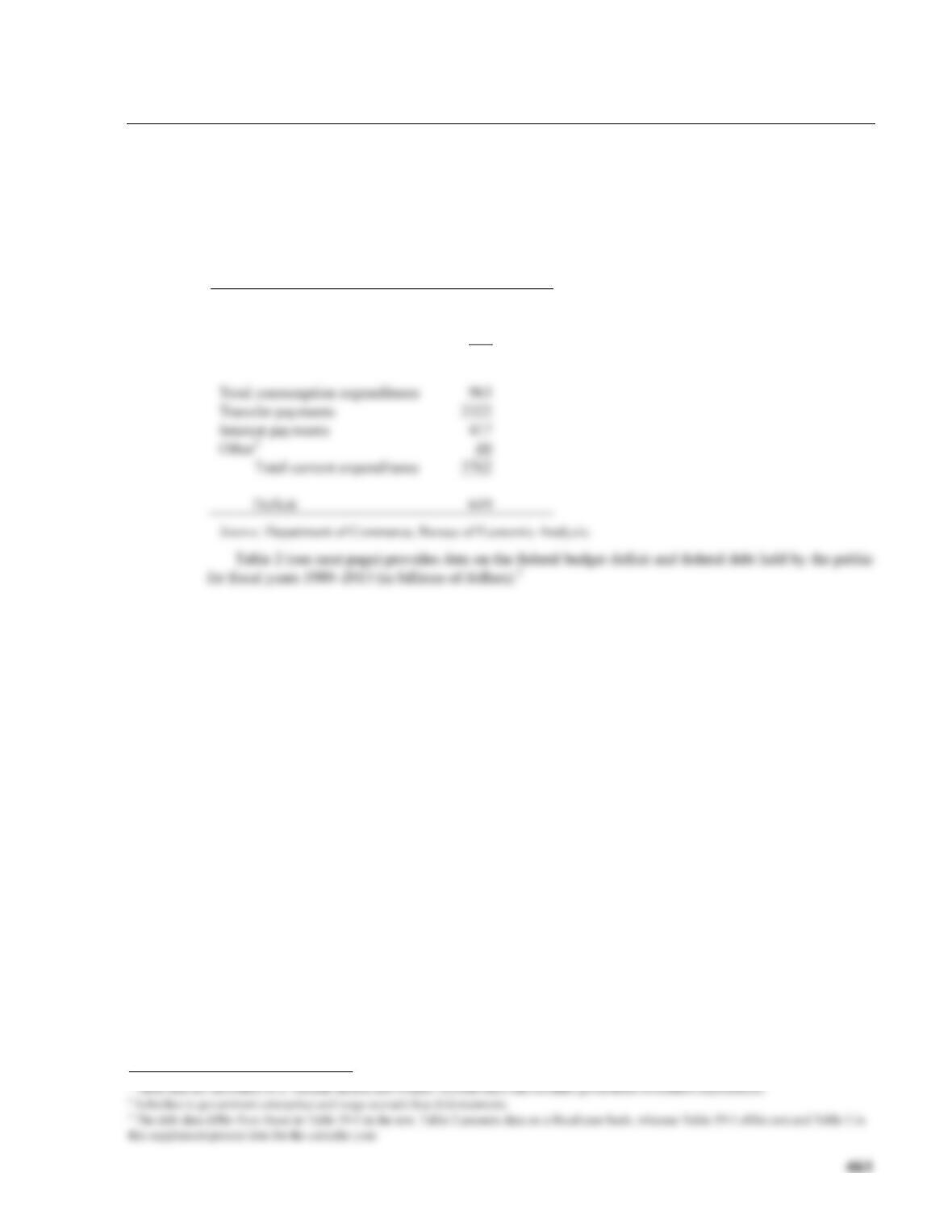
interest payments on the national debt. Table 1 provides revenues and expenditures for 2013 (in billions of
dollars).1
Table 1 Federal Receipts and Expenditures
Income taxes
1287
Social Security
1092
Other (including corporate)
734
Total receipts
3113
963
2322
Interest payments
417
Total current expenditures
3762
649
1 These data are calculated on a National Income and Product Account basis that excludes government investment expenditures.
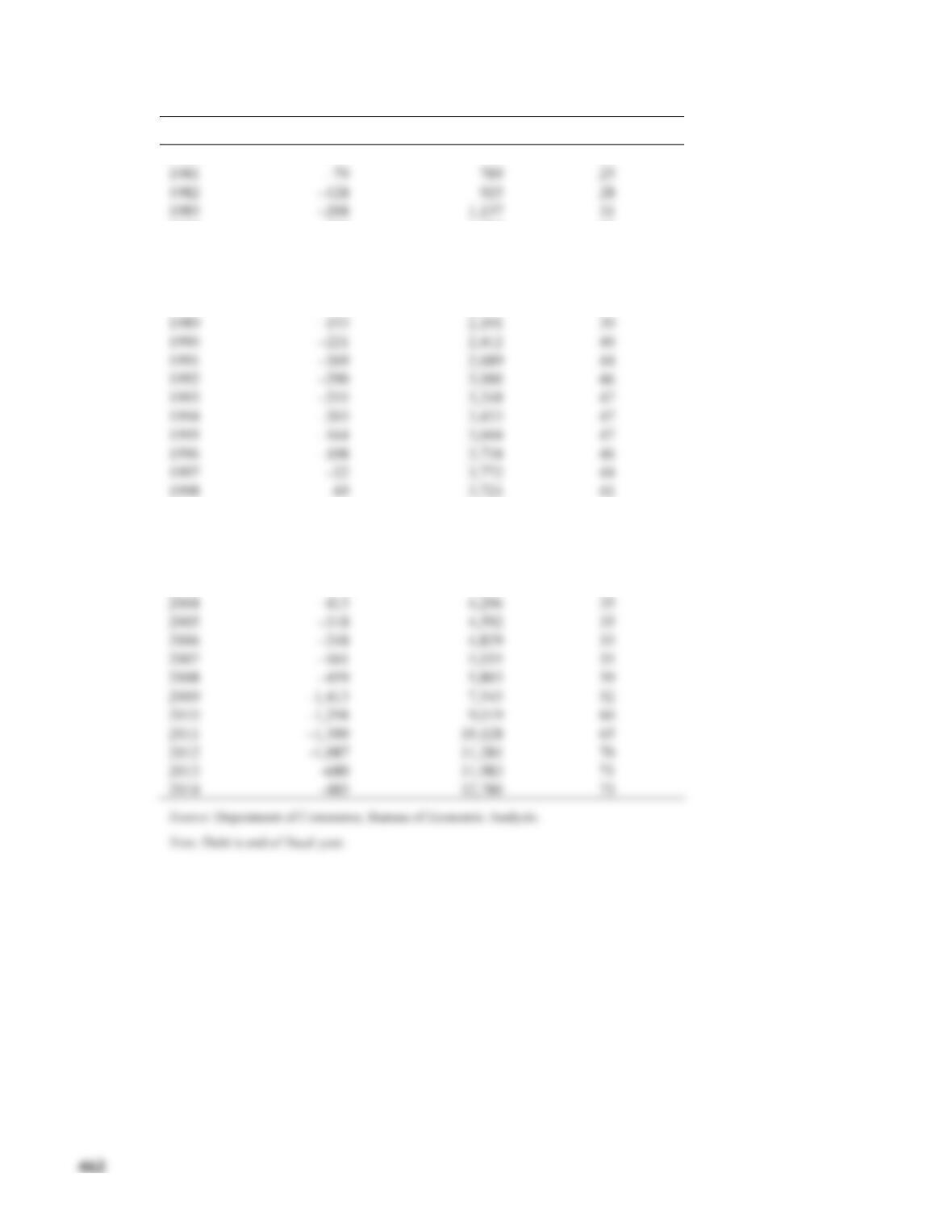
Table 2 Federal Budget Deficit and Debt
Year
Deficit (–)/Surplus (+)
Debt
Debt/GDP (%)
1980
–74
712
25
1981
–79
789
25
1982
–128
925
28
1983
–208
1,137
31
1984
–185
1,307
32
1985
–212
1,507
35
1986
–221
1,741
38
1987
–150
1,890
39
1988
–155
2,052
39
1989
–153
2,191
39
1990
–221
2,412
40
1991
–269
2,689
44
1992
–290
3,000
46
1993
–255
3,248
47
1994
–203
3,433
47
1995
–164
3,604
47
1996
–108
3,734
46
1997
–22
3,772
44
1998
3,721
41
1999
126
3,632
38
2000
236
3,410
33
2001
128
3,320
31
2002
–158
3,540
32
2003
–378
3,913
34
2004
–413
4,296
35
2005
–318
4,592
35
2006
–248
4,829
35
2007
–161
5,035
35
2008
–459
5,803
39
2009
7,545
52
2010
9,019
60
2011
65
2012
70
2013
71
2014
73
CASE STUDY EXTENSION
19–2 How Important Is Crowding Out?
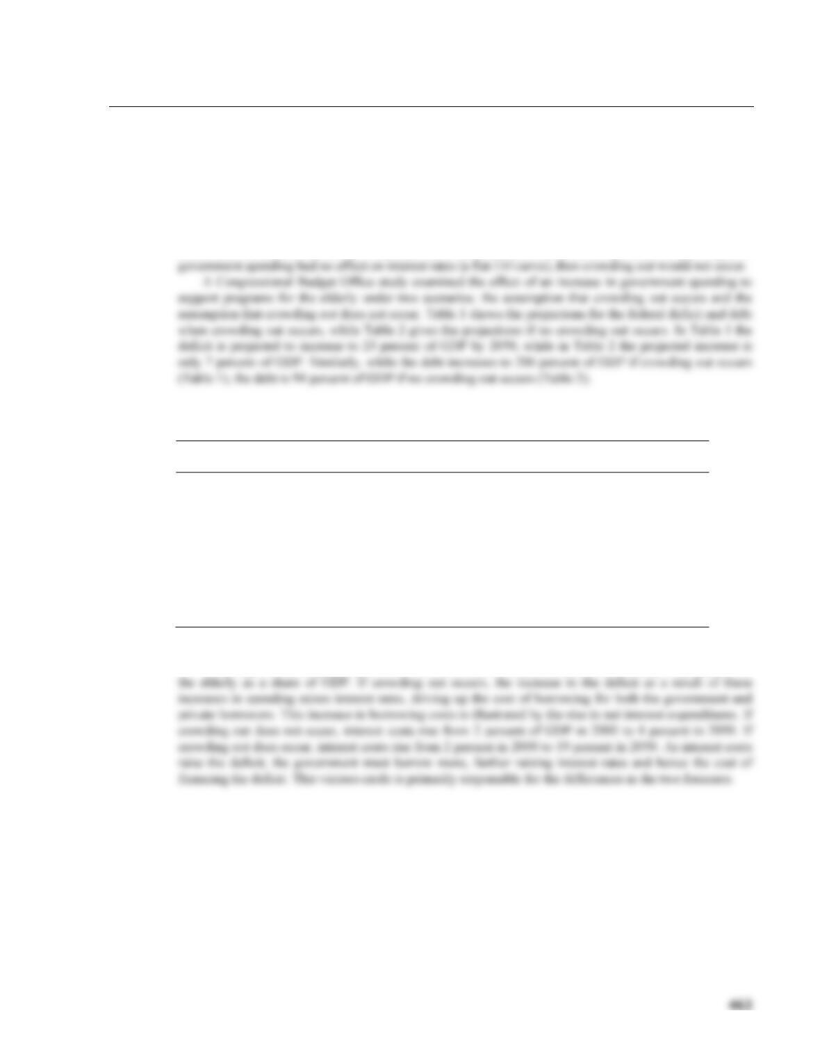
Projections of future deficits should take into account the crowding–out effect of expansionary fiscal
policies. Both the direct rise in interest rates and the dampening effect on output tend to increase the
deficit. This occurs because higher interest rates increase the cost of financing existing debt, and less
expansion in output (and incomes) means lower taxes than otherwise.
As the IS–LM analysis indicates, expansionary government policy (running deficits) shifts the IS
curve outward, increasing aggregate demand. However, because the increase in government spending
raises interest rates, it “crowds out” some private investment and hence diminishes the effect on output. If
Table 1 Projections of Federal Receipts and Expenditures with Economic Feedback (percentage
of GDP)
2000
2010
2020
2030
2040
2050
Receipts
21
20
20
20
20
20
Expenditures
21
20
22
25
30
43
Consumption
5
4
4
4
4
4
Transfers, grants, and subsidies
Social Security
4
5
6
6
7
7
Medicare
3
4
5
6
7
7
Other
6
6
6
6
7
7
Net interest
2
1
1
2
6
19
Deficit (–) or surplus
0
1
–1
–5
–10
–23
Debt held by the public
42
21
17
40
93
206
Source: Long–Term Budgetary Pressures and Policy Options, Congressional Budget Office, May 1998, Table 2–1.
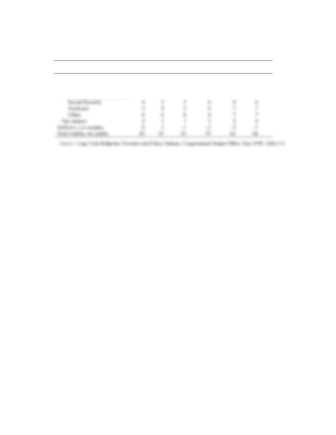
What explains these differences? Both scenarios show similar increases in spending on programs for
464
Table 2 Projections of Federal Receipts and Expenditures without Economic Feedback (percentage
of GDP)
2000
2010
2020
2030
2040
2050
Receipts
21
20
20
20
20
20
Expenditures
21
19
21
24
26
27
Consumption
5
4
4
4
4
4
Transfers, grants, and subsidies
Social Security
Medicare
Other
Net interest
42
21
15
32
61
94