Basic Econometrics, Gujarati and Porter
207
CHAPTER 19:
THE IDENTIFICATION PROBLEM
19.1 Using the definitions of M, m, K, and k, and letting R equal
the number of variables (endogenous as well as predetermined)
19.2
The structural coefficients are:
0 3 1 0 0 3 1 0
β π β π α π α π
= − = −
19.3
(a) The reduced form equations are:
0 1
(1)
t t t
Y I w
π π
= + +
(b) The reduced form equations are:
(1)
W UN M w
π π π
= + + +
(c) This problem is designed to show the tedious nature of
19.4
See Exercise 19.3. The rank condition test provides the same result.
208
19.6
(a) For this system, M = 2 (Y
, Y2) and K = 2 (X
, X
). By the order
19.7
(a) Following the system (19.2.12) and (19.2.22), it can be shown
that:
(
b
) To test this hypothesis, we need the standard error of
ˆ
γ
. But as
19.8
(
a
) In this example,
Y
1
is not identified but
Y
2
is. This system is
similar to the system (19.2.12) and (19.2.13). Thus,
19.11
Here
M
= 5 and
K
= 4. By the order condition,
1 2 5
, ,and
Y Y Y
are
just identified,
Y
3
is not identified and
Y
4
is overidentified.
209
19.12
For this model,
M
= 4 and
K
= 2. By the order condition,
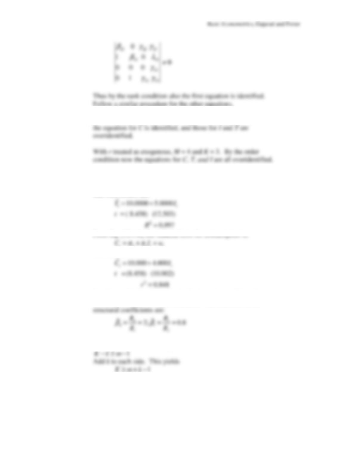
19.13
From Eq. (19.1.2), the reduced form of the income equation is:
0 1
t t t
Y I u
π π
= + +
The OLS results are:
2 3
t t t
The OLS results are:
For this model, M = 2 and K = 1. By the order condition, the
consumption function is just identified. The estimates of the
19.14
See Exercise 19.1. From Eq. (19.3.1), with Definition 19.2,
19.15
(
a
) The reduced form equations are:
Basic Econometrics, Gujarati and Porter
Empirical Exercises
19.16
(
a
) & (
b
) Here
M
= 2 and
K
= 2. By the order condition, the demand
function is not identified and the supply function is overidentified.
The
Stata
results of this exercise are as follows:
Source | SS df MS Number of obs = 37
——————————————————————————
m2 | Coef. Std. Err. t P>|t| [95% Conf. Interval]
————-+————-——————————-——————–
——————————————————————————
Basic Econometrics, Gujarati and Porter
211
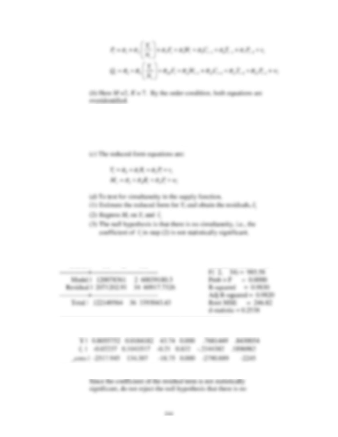
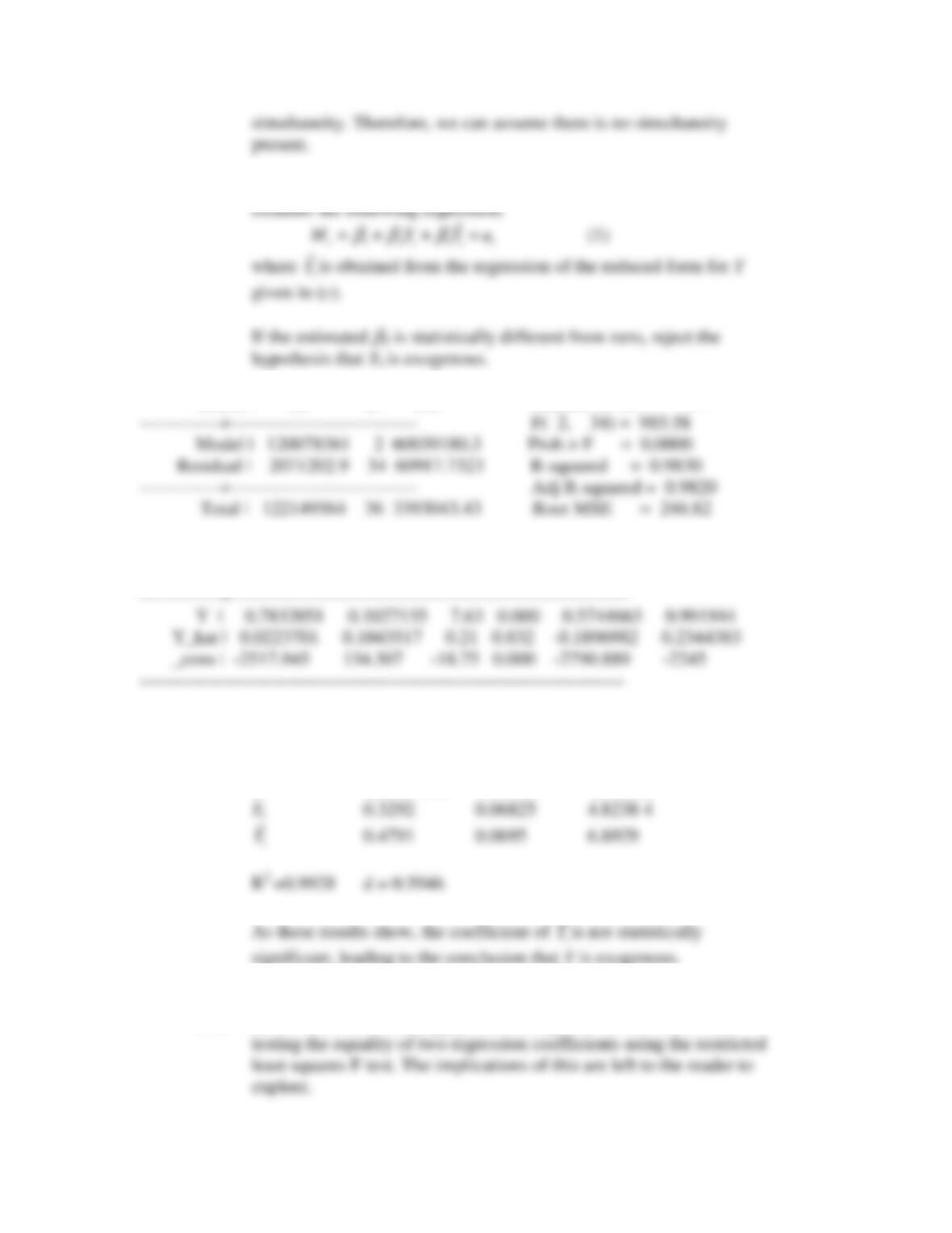
(
e
) Here we use the exogeneity test discussed in the chapter. We
Source | SS df MS Number of obs = 37
——————————————————————————
m2 | Coef. Std. Err. t P>|t| [95% Conf. Interval]
Dependent Variable: M2
Variable Coefficient Std. Error t-Statistic
C -2295.7898 78.9873 -29.0652
19.17
(a) To test this, we can apply the techniques from Section 8.7 for

Basic Econometrics, Gujarati and Porter
212
(b) To see if
ˆ
t
ν
is correlated with
u
2t
, we can treat
ˆ
t
ν
as a regressor